4.7 Testing a Null Hypothesis with an Exact Approach or Bootstrapping
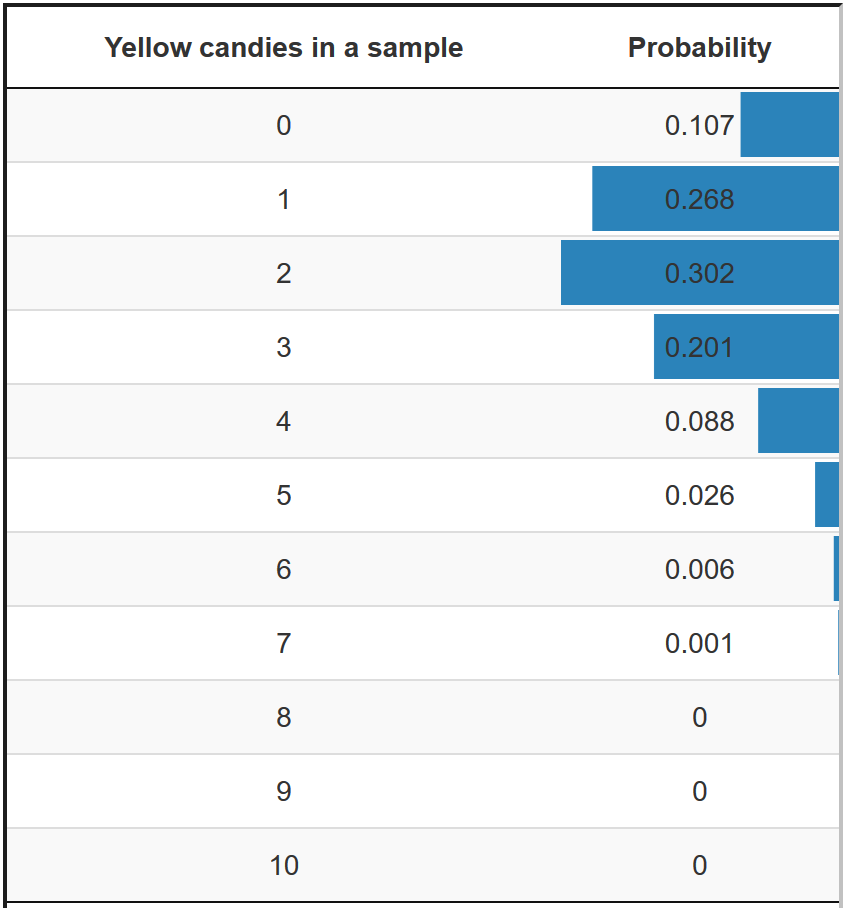
Exact approaches calculate probabilities for discrete outcomes. In the candy example, the number of yellow candies in a sample bag of ten candies is a discrete outcome. With the binomial formula, the exact probability of zero yellow candies can be calculated, the probability of one yellow candy, two yellow candies, and so on (see Figure 4.21).

Figure 4.21: Probabilities of a sample with a particular number of yellow candies if 20 per cent of the candies are yellow in the population.
Let us imagine that our sample bag of ten candies contains six yellow candies and we hypothesize that twenty per cent of the candies are yellow in the population. The p value of our sample outcome (six yellow candies) sums the probabilities of drawing a sample bag with six, seven, eight, nine, or ten yellow candies from a population in which twenty per cent of the candies are yellow (our null hypothesis). The p value happens to be (around) .007 (.006 + .001 + 0 + 0 + 0). This is the right-sided p value if we assume that our hypothesis is true.
With the p value, we perform the significance test as usual. The p value is well below the significance level of .05, so we reject the null hypothesis that twenty per cent of all candies in the population are yellow.
The situation is slightly more complicated if we want to execute a significance test with a sampling distribution created with bootstrapping. To understand the testing procedure with bootstrapping, we first have to discuss the relation between null-hypothesis testing and confidence intervals.
4.7.1 Relation between null-hypothesis tests and confidence intervals
Figure 4.22 shows media literacy scores in a random sample of children and their average media literacy score (red). The hypothesized average media literacy in the population of children is shown on the top axis. The curve represents the sampling distribution if the null hypothesis is true.
Figure 4.22: How does null hypothesis significance relate to confidence intervals?
Do you remember how we constructed a confidence interval in Chapter 3, Section ??? We looked for all population values for which the sample outcome is sufficiently plausible. Sufficiently plausible means that our observed sample outcome is among the sample outcomes that are closest to the population value. By convention, we use a confidence level of 95 per cent, which means that our observed sample is among the 95 per cent of all samples that have outcomes closest to the population value.
But wait a minute. If the sample outcome is among the 95 per cent of samples in the middle of the sampling distribution, it is NOT among the extreme five percent of all samples. This is simply another way of saying that the observed sample outcome is not statistically significant at the five per cent significance level. A 95% confidence interval contains all null hypothesis values for which our sample outcome is not statistically significant at the 5% significance level. Confidence levels and significance levels are related.
If we know the 95% confidence interval, we can immediately see if our null hypothesis must be rejected or not. If the population value in our null hypothesis lies within the 95% confidence interval, the null hypothesis is NOT rejected. The sample that we have drawn is sufficiently plausible if our null hypothesis is true. In contrast, we must reject the null hypothesis if the hypothesized population value is NOT in the 95% confidence interval.
Let us assume, for example, that average media literacy in our sample is 3.0 and that the 95% confidence interval for average media literacy ranges from 1.0 to 5.0. A null hypothesis specifying 2.5 as population average must not be rejected at the five percent significance level because 2.5 is in between 1.0 and 5.0, that is, inside the 95% confidence interval. If our null hypothesis says that average media literacy in the population is 5.5, we must reject this null hypothesis because it is outside the 95% confidence interval. The null hypothesis that average media literacy in the population is 0.0 must be rejected for the same reason.
Note that the hypothesized value can be too high or too low for the confidence interval, so a hypothesis test using a confidence interval is two-sided.
4.7.2 Testing a null hypothesis with bootstrapping
Using the confidence interval is the easiest and sometimes the only way of testing a null hypothesis if we create the sampling distribution with bootstrapping. For instance, we may use the median as the preferred measure of central tendency rather than the mean if the distribution of scores is quite skewed and the sample is not very large. In this situation, a theoretical probability distribution for the sample median is not known, so we resort to bootstrapping.
Bootstrapping creates an empirical sampling distribution: a lot of samples with a median calculated for each sample. A confidence interval can be created from this sampling distribution (see Section 3.5.3). If our null hypothesis about the population median is included in the 95% confidence interval, we do not reject the null hypothesis. Otherwise, we reject it.
For the lovers of details, we add a disclaimer. A confidence interval contains all null hypotheses not rejected by our current sample if we use a normal distribution (Jerzy Neyman, 1937: 376-378), but this is not always the case if we calculate the confidence interval with the critical values of a t distribution (see, for example, Smithson, 2001) or if we use a bootstrapped confidence interval. In these cases, null hypothesis values near the interval boundaries may or may not be rejected by our current sample; we do not know. A confidence interval gives us an approximate range of null hypotheses that are not rejected by our sample rather than an exact range.