Chapter 6 Moderation with Analysis of Variance (ANOVA)
Key concepts: eta-squared, between-groups variance, within-groups variance, F test on analysis of variance model, pairwise comparisons, post-hoc tests, one-way analysis of variance, two-way analysis of variance, balanced design, main effects, moderation, interaction effect.
Watch this micro lecture on moderation with analysis of variance for an overview of the chapter.
Summary
Imagine an experiment in which participants watch a video promoting a charity. They see George Clooney, Angelina Jolie, or no celebrity endorse the charity’s fund-raiser. Afterwards, their willingness to donate to the charity is measured. Which campaign works best, that is, produces highest average willingness to donate? Or does one campaign work better for females, another for males?
In this example, we want to compare the outcome scores (average willingness to donate) across more than two groups (participants who saw Clooney, Jolie, or no celebrity). To this end, we use analysis of variance. The null hypothesis tested in analysis of variance states that all groups have the same average outcome score in the population.
This null hypothesis is similar to the one we test in an independent-samples t test for two groups. With three or more groups, we must use the variance of the group means (between-groups variance) to test the null hypothesis. If the between-groups variance is zero, all group means are equal.
In addition to between-groups variance, we have to take into account the variance of outcome scores within groups (within-groups variance). Within-groups variance is related to the fact that we may obtain different group means even if we draw random samples from populations with the same means. The ratio of between-groups variance over within-groups variance gives us the F test statistic, which has an F distribution.
Differences in average outcome scores for groups on one independent variable (usually called factor in analysis of variance) are called a main effect. A main effect represents an overall or average effect of a factor. If we have only one factor in our model, for instance, the endorser of the fund-raiser, we apply a one-way analysis of variance. With two factors, we have a two-way analysis of variance, and so on.
With two or more factors, we can have interaction effects in addition to main effects. An interaction effect is the joint effect of two or more factors on the dependent variable. An interaction effect is best understood as different effects of one factor across different groups on another factor. For example, Clooney may increase willingness to donate among females but Jolie works best for males.
The phenomenon that a variable can have different effects for different groups on another variable is called moderation. We usually think of one factor as the predictor (or independent variable) and the other factor as the moderator. The moderator (e.g., sex) changes the effect of the predictor (e.g., celebrity endorser) on the dependent variable (e.g., willingness to donate).
Essential Analytics
In SPSS, we use the One-Way ANOVA option in the Compare Means submenu for one-way analysis of variance and the Univariate option in the General Linear Model submenu for two-way analysis of variance.

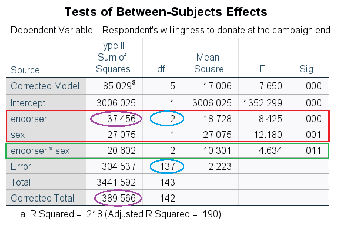
Figure 6.1: SPSS table of main and interaction effects in a two-way analysis of variance.
The significance tests on the main effects and interaction effect are reported in the Tests of Between-Subjects Effects table. Figure 6.1 offers an example. The tests on the main effects are in the red box and the green box contains the test on the interaction effect. The APA-style summary of the main effect of endorser is: F (2, 137) = 8.43, p < .001, eta2 = .10. Note the two degrees of freedom in between the brackets, which are marked by a blue ellipse in the figure. You get the effect size eta2 by dividing the sum of squares of an effect by the corrected total sum of squares (in purple ellipses in the figure): 37.456 / 389.566 = 0.10.
Interpret the effects by comparing mean scores on the dependent variable among groups:
If there are two groups on a factor, for example, females and males, compare the two group means: Which group scores higher? For example, females score on average 5.05 on willingness to donate whereas the average willingness is only 4.19 for males. The F test shows whether or not the difference between the two groups is statistically significant.
If a factor has more than two groups, for example, Jolie, Clooney, and no celebrity endorser, use post-hoc comparisons with Bonferroni correction. The results tell you which group scores on average higher than another group and whether the difference is statistically significant if we correct for capitalization on chance.
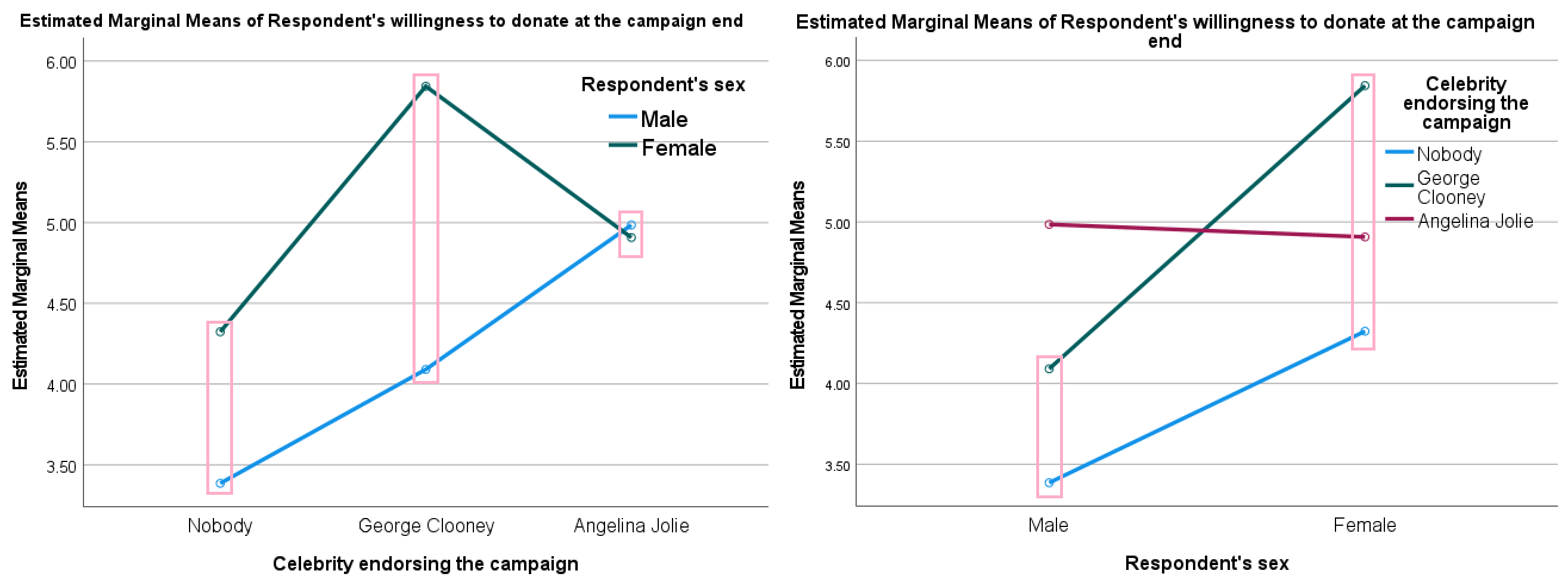
If you want to interpret an interaction effect, create means plots such as Figure 6.2. Compare the differences between means across groups. In the left panel, for example, we see that the effect of sex on willingness to donate (the difference between the mean score of females and the mean score of males) is larger for Clooney (pink box in the middle) than for no celebrity endorser (pink box on the left), and it is smallest for Angelina Jolie (pink box on the right). Similarly, we see that the effect of seeing Clooney instead of no celebrity endorser is larger for females (right-hand panel, pink box on the right) than for males (right-hand panel, pink box on the left).

Figure 6.2: SPSS means plots of the interaction effect of sex and endorser on willingness to donate. Note that the pink boxes have been added manually to aid the interpretation.