Probability Models
Why do we need them
Exact approach
Applicable
Exact probabilities can only be calculated for:
- Discreet variables
- Categorical variables
An exact approach lists and counts all possible combinations.
Coin values
Coin values for heads and tails.
\(\{1, 0\}\)
10 tosses
| Toss1 | Toss2 | Toss3 | Toss4 | Toss5 | Toss6 | Toss7 | Toss8 | Toss9 | Toss10 |
|---|---|---|---|---|---|---|---|---|---|
| 0.5 | 0.5 | 0.5 | 0.5 | 0.5 | 0.5 | 0.5 | 0.5 | 0.5 | 0.5 |
| 0.5 | 0.5 | 0.5 | 0.5 | 0.5 | 0.5 | 0.5 | 0.5 | 0.5 | 0.5 |
| 0.5 | 0.5 | 0.5 | 0.5 | 0.5 | 0.5 | 0.5 | 0.5 | 0.5 | 0.5 |
| 0.5 | 0.5 | 0.5 | 0.5 | 0.5 | 0.5 | 0.5 | 0.5 | 0.5 | 0.5 |
| 0.5 | 0.5 | 0.5 | 0.5 | 0.5 | 0.5 | 0.5 | 0.5 | 0.5 | 0.5 |
| 0.5 | 0.5 | 0.5 | 0.5 | 0.5 | 0.5 | 0.5 | 0.5 | 0.5 | 0.5 |
| 0.5 | 0.5 | 0.5 | 0.5 | 0.5 | 0.5 | 0.5 | 0.5 | 0.5 | 0.5 |
| Toss1 | Toss2 | Toss3 | Toss4 | Toss5 | Toss6 | Toss7 | Toss8 | Toss9 | Toss10 | probability |
|---|---|---|---|---|---|---|---|---|---|---|
| 0.5 | 0.5 | 0.5 | 0.5 | 0.5 | 0.5 | 0.5 | 0.5 | 0.5 | 0.5 | 0.0009766 |
| 0.5 | 0.5 | 0.5 | 0.5 | 0.5 | 0.5 | 0.5 | 0.5 | 0.5 | 0.5 | 0.0009766 |
| 0.5 | 0.5 | 0.5 | 0.5 | 0.5 | 0.5 | 0.5 | 0.5 | 0.5 | 0.5 | 0.0009766 |
| 0.5 | 0.5 | 0.5 | 0.5 | 0.5 | 0.5 | 0.5 | 0.5 | 0.5 | 0.5 | 0.0009766 |
| 0.5 | 0.5 | 0.5 | 0.5 | 0.5 | 0.5 | 0.5 | 0.5 | 0.5 | 0.5 | 0.0009766 |
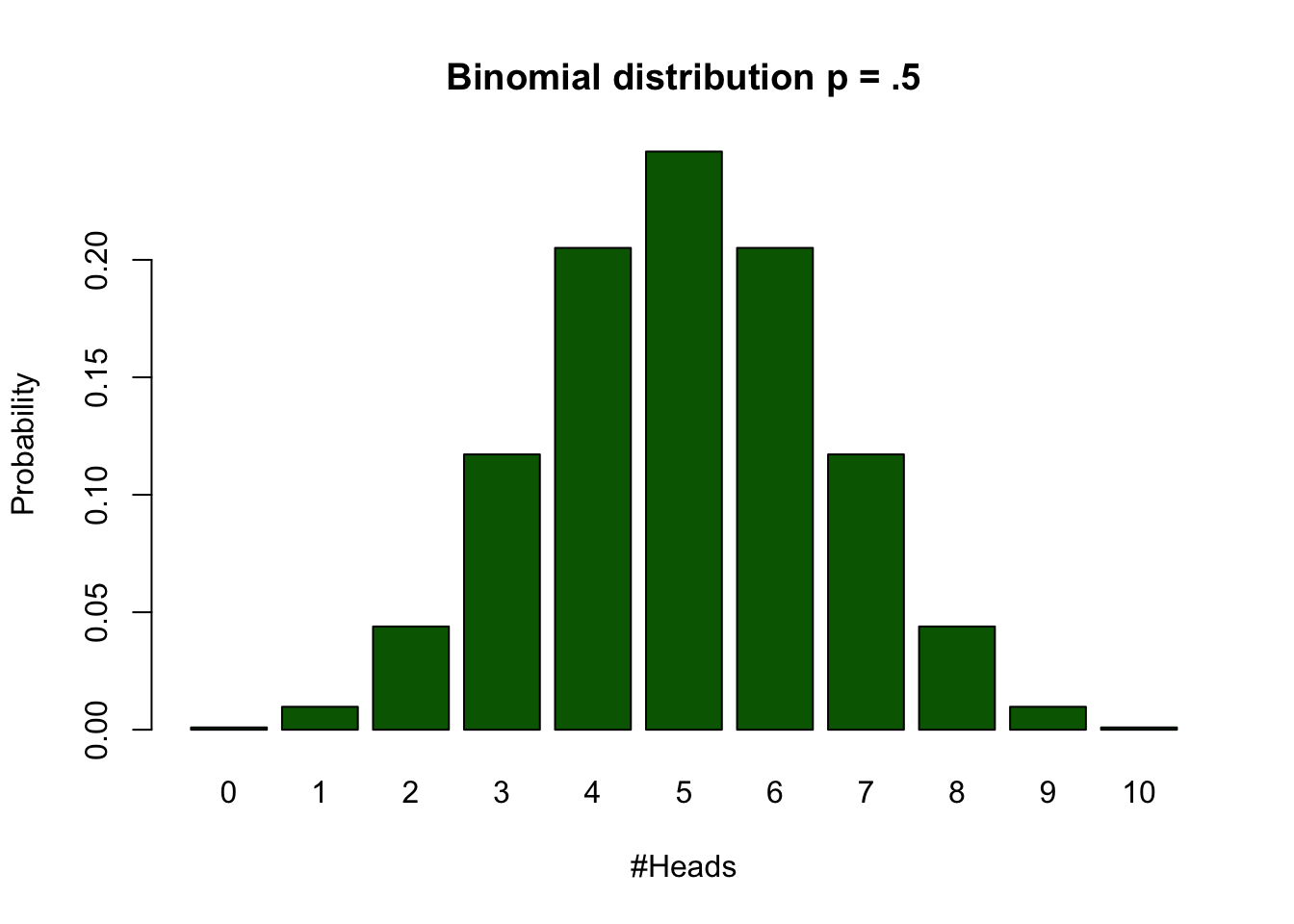
| #Heads | frequencies | Probabilities |
|---|---|---|
| 0 | 1 | 0.0009766 |
| 1 | 10 | 0.0097656 |
| 2 | 45 | 0.0439453 |
| 3 | 120 | 0.1171875 |
| 4 | 210 | 0.2050781 |
| 5 | 252 | 0.2460938 |
| 6 | 210 | 0.2050781 |
| 7 | 120 | 0.1171875 |
| 8 | 45 | 0.0439453 |
| 9 | 10 | 0.0097656 |
| 10 | 1 | 0.0009766 |
Calculate binomial probabilities
\[ {n\choose k}p^k(1-p)^{n-k}, \small {n\choose k} = \frac{n!}{k!(n-k)!} \]
n = 10   # Sample size
k = 0:10 # Discrete probability space
p = .5 # Probability of head| n | k | p | n! | k! | (n-k)! | (n over k) | p^k | (1-p)^(n-k) | Binom Prob |
|---|---|---|---|---|---|---|---|---|---|
| 10 | 0 | 0.5 | 3628800 | 1 | 3628800 | 1 | 1.0000000 | 0.0009766 | 0.0009766 |
| 10 | 1 | 0.5 | 3628800 | 1 | 362880 | 10 | 0.5000000 | 0.0019531 | 0.0097656 |
| 10 | 2 | 0.5 | 3628800 | 2 | 40320 | 45 | 0.2500000 | 0.0039063 | 0.0439453 |
| 10 | 3 | 0.5 | 3628800 | 6 | 5040 | 120 | 0.1250000 | 0.0078125 | 0.1171875 |
| 10 | 4 | 0.5 | 3628800 | 24 | 720 | 210 | 0.0625000 | 0.0156250 | 0.2050781 |
| 10 | 5 | 0.5 | 3628800 | 120 | 120 | 252 | 0.0312500 | 0.0312500 | 0.2460938 |
| 10 | 6 | 0.5 | 3628800 | 720 | 24 | 210 | 0.0156250 | 0.0625000 | 0.2050781 |
| 10 | 7 | 0.5 | 3628800 | 5040 | 6 | 120 | 0.0078125 | 0.1250000 | 0.1171875 |
| 10 | 8 | 0.5 | 3628800 | 40320 | 2 | 45 | 0.0039063 | 0.2500000 | 0.0439453 |
| 10 | 9 | 0.5 | 3628800 | 362880 | 1 | 10 | 0.0019531 | 0.5000000 | 0.0097656 |
| 10 | 10 | 0.5 | 3628800 | 3628800 | 1 | 1 | 0.0009766 | 1.0000000 | 0.0009766 |
Warning
Formula not exam material
Binomial distribution
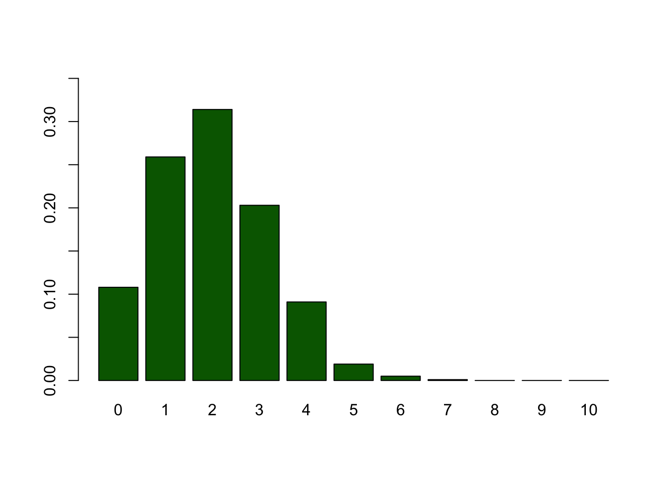
Bootstrapping
Sampling from your sample to approximate the sampling distribution.
My Coin tosses
my.tosses = c(0,0,1,0,0,0,0,0,1,0)Sample from the sample
Sampling with replacement
sample(my.tosses, replace = TRUE) [1] 0 0 0 1 0 0 0 0 0 0sample(my.tosses, replace = TRUE) [1] 1 0 0 0 0 0 1 0 0 0sample(my.tosses, replace = TRUE) [1] 0 0 0 0 0 0 0 0 0 0sample(my.tosses, replace = TRUE) [1] 0 0 0 0 0 1 0 0 0 0Sampling from the sample
n.bootstrap.samples = 1000
n.heads = vector()

for (i in 1:n.bootstrap.samples) {
  bootstrap.sample <- sample(my.tosses, replace = TRUE)

  n.heads[i] <- sum(bootstrap.sample)
}| 2 | 1 | 1 | 2 | 3 | 5 | 3 | 2 | 3 | 2 | 3 | 3 | 5 | 2 | 0 | 0 | 1 | 2 | 3 | 1 | 1 | 0 | 4 | 1 | 4 | 2 | 3 | 1 | 2 | 4 | 2 | 3 | 2 | 1 | 3 | 2 | 3 | 0 | 3 | 2 |
| 2 | 4 | 2 | 1 | 1 | 1 | 2 | 1 | 4 | 2 | 2 | 4 | 3 | 1 | 2 | 0 | 3 | 1 | 1 | 4 | 3 | 1 | 1 | 2 | 3 | 1 | 3 | 2 | 2 | 2 | 3 | 2 | 3 | 4 | 0 | 2 | 2 | 0 | 2 | 1 |
| 1 | 1 | 3 | 2 | 1 | 4 | 3 | 1 | 2 | 3 | 1 | 0 | 2 | 2 | 2 | 1 | 0 | 2 | 3 | 2 | 2 | 2 | 2 | 2 | 3 | 1 | 0 | 1 | 2 | 1 | 4 | 3 | 2 | 2 | 2 | 2 | 2 | 2 | 1 | 0 |
| 3 | 1 | 2 | 1 | 2 | 5 | 1 | 3 | 1 | 4 | 4 | 0 | 1 | 2 | 1 | 2 | 4 | 1 | 0 | 2 | 3 | 1 | 1 | 2 | 2 | 1 | 5 | 2 | 3 | 3 | 2 | 1 | 3 | 3 | 3 | 4 | 1 | 0 | 2 | 2 |
| 2 | 2 | 1 | 2 | 3 | 4 | 0 | 0 | 3 | 7 | 2 | 3 | 3 | 5 | 3 | 3 | 2 | 1 | 1 | 3 | 1 | 3 | 3 | 2 | 1 | 2 | 4 | 1 | 1 | 0 | 1 | 1 | 2 | 2 | 2 | 4 | 2 | 1 | 1 | 4 |
| 2 | 3 | 1 | 1 | 4 | 1 | 2 | 2 | 2 | 2 | 1 | 1 | 1 | 2 | 1 | 0 | 3 | 2 | 4 | 4 | 4 | 2 | 2 | 0 | 3 | 3 | 2 | 0 | 3 | 2 | 2 | 2 | 1 | 1 | 3 | 2 | 1 | 0 | 1 | 3 |
| 2 | 2 | 2 | 2 | 2 | 2 | 2 | 1 | 2 | 2 | 1 | 3 | 1 | 3 | 4 | 2 | 1 | 2 | 4 | 3 | 2 | 1 | 1 | 1 | 5 | 0 | 0 | 3 | 2 | 0 | 0 | 2 | 5 | 2 | 0 | 2 | 1 | 1 | 4 | 1 |
| 1 | 3 | 2 | 1 | 5 | 2 | 0 | 1 | 4 | 2 | 1 | 2 | 4 | 0 | 4 | 0 | 1 | 3 | 4 | 1 | 3 | 2 | 5 | 3 | 4 | 3 | 2 | 2 | 2 | 1 | 0 | 1 | 0 | 4 | 3 | 1 | 3 | 3 | 3 | 0 |
| 1 | 4 | 1 | 2 | 2 | 3 | 3 | 0 | 2 | 0 | 2 | 3 | 1 | 1 | 2 | 2 | 1 | 4 | 2 | 1 | 0 | 2 | 2 | 2 | 2 | 1 | 1 | 1 | 2 | 0 | 3 | 0 | 1 | 1 | 1 | 0 | 2 | 3 | 4 | 2 |
| 1 | 1 | 2 | 1 | 2 | 1 | 3 | 0 | 4 | 2 | 0 | 0 | 1 | 3 | 1 | 0 | 1 | 4 | 1 | 3 | 1 | 3 | 2 | 3 | 2 | 1 | 1 | 1 | 3 | 2 | 2 | 1 | 1 | 1 | 1 | 1 | 1 | 0 | 0 | 2 |
| 3 | 2 | 3 | 0 | 1 | 1 | 0 | 0 | 3 | 2 | 3 | 4 | 6 | 2 | 1 | 0 | 3 | 2 | 4 | 3 | 2 | 2 | 1 | 1 | 1 | 1 | 4 | 1 | 1 | 3 | 1 | 3 | 2 | 1 | 2 | 3 | 2 | 1 | 0 | 2 |
| 1 | 3 | 2 | 2 | 1 | 3 | 2 | 5 | 0 | 2 | 3 | 2 | 2 | 2 | 1 | 1 | 4 | 1 | 2 | 0 | 2 | 1 | 2 | 3 | 3 | 1 | 5 | 1 | 1 | 1 | 1 | 2 | 3 | 3 | 1 | 1 | 0 | 2 | 3 | 0 |
| 3 | 2 | 2 | 2 | 1 | 0 | 2 | 1 | 0 | 3 | 3 | 2 | 2 | 2 | 2 | 1 | 0 | 3 | 4 | 1 | 2 | 2 | 2 | 1 | 0 | 1 | 3 | 2 | 3 | 0 | 3 | 2 | 2 | 5 | 2 | 2 | 3 | 2 | 1 | 1 |
| 2 | 1 | 3 | 2 | 2 | 1 | 4 | 2 | 1 | 4 | 1 | 3 | 0 | 0 | 2 | 1 | 2 | 2 | 4 | 2 | 2 | 3 | 0 | 4 | 2 | 1 | 1 | 2 | 2 | 2 | 1 | 0 | 2 | 0 | 3 | 1 | 2 | 5 | 2 | 0 |
| 3 | 3 | 3 | 1 | 2 | 2 | 2 | 3 | 3 | 2 | 1 | 3 | 4 | 0 | 2 | 2 | 1 | 2 | 1 | 2 | 1 | 4 | 4 | 4 | 2 | 0 | 2 | 3 | 2 | 3 | 1 | 3 | 5 | 5 | 3 | 1 | 2 | 4 | 2 | 1 |
| 3 | 1 | 1 | 0 | 1 | 4 | 1 | 1 | 3 | 0 | 2 | 3 | 4 | 4 | 3 | 1 | 1 | 2 | 2 | 0 | 1 | 2 | 1 | 1 | 3 | 6 | 1 | 2 | 3 | 4 | 2 | 4 | 3 | 2 | 2 | 1 | 6 | 4 | 3 | 4 |
| 2 | 1 | 3 | 0 | 2 | 2 | 2 | 1 | 1 | 2 | 3 | 4 | 4 | 2 | 2 | 3 | 1 | 2 | 4 | 2 | 4 | 3 | 1 | 2 | 2 | 2 | 1 | 1 | 4 | 1 | 3 | 0 | 2 | 2 | 2 | 2 | 3 | 4 | 2 | 0 |
| 0 | 3 | 2 | 1 | 3 | 3 | 2 | 3 | 1 | 3 | 0 | 3 | 3 | 2 | 2 | 3 | 1 | 0 | 2 | 1 | 0 | 1 | 4 | 1 | 2 | 2 | 2 | 2 | 5 | 3 | 1 | 1 | 1 | 1 | 1 | 3 | 3 | 1 | 3 | 6 |
| 0 | 2 | 4 | 2 | 2 | 3 | 2 | 2 | 2 | 3 | 3 | 2 | 2 | 2 | 3 | 1 | 0 | 1 | 3 | 3 | 3 | 2 | 2 | 2 | 1 | 2 | 3 | 1 | 3 | 2 | 3 | 0 | 3 | 2 | 3 | 0 | 3 | 4 | 4 | 3 |
| 0 | 1 | 1 | 2 | 1 | 0 | 4 | 2 | 3 | 1 | 1 | 1 | 2 | 2 | 2 | 2 | 4 | 1 | 3 | 4 | 1 | 2 | 2 | 1 | 2 | 3 | 1 | 1 | 1 | 3 | 3 | 3 | 3 | 1 | 0 | 2 | 1 | 3 | 1 | 2 |
| 3 | 2 | 2 | 3 | 2 | 1 | 1 | 4 | 1 | 2 | 1 | 3 | 3 | 1 | 1 | 2 | 3 | 2 | 0 | 1 | 0 | 1 | 0 | 3 | 3 | 1 | 4 | 1 | 6 | 4 | 2 | 3 | 3 | 3 | 1 | 4 | 2 | 1 | 2 | 4 |
| 0 | 2 | 0 | 1 | 3 | 2 | 1 | 2 | 4 | 2 | 3 | 2 | 0 | 1 | 3 | 0 | 2 | 1 | 0 | 4 | 4 | 0 | 3 | 5 | 4 | 1 | 3 | 2 | 3 | 1 | 1 | 3 | 1 | 1 | 2 | 2 | 1 | 2 | 0 | 4 |
| 2 | 1 | 2 | 1 | 2 | 3 | 2 | 3 | 0 | 3 | 1 | 4 | 0 | 2 | 3 | 3 | 2 | 1 | 4 | 2 | 1 | 1 | 1 | 1 | 2 | 4 | 4 | 3 | 3 | 2 | 2 | 2 | 2 | 3 | 2 | 2 | 4 | 0 | 2 | 1 |
| 2 | 3 | 2 | 3 | 2 | 2 | 1 | 2 | 2 | 2 | 2 | 0 | 3 | 2 | 4 | 4 | 3 | 0 | 1 | 3 | 2 | 3 | 1 | 3 | 3 | 0 | 0 | 3 | 1 | 1 | 4 | 2 | 3 | 2 | 3 | 4 | 2 | 3 | 1 | 1 |
| 1 | 0 | 1 | 5 | 3 | 3 | 3 | 2 | 4 | 5 | 2 | 3 | 0 | 0 | 0 | 2 | 0 | 1 | 2 | 3 | 2 | 2 | 0 | 2 | 3 | 2 | 2 | 1 | 0 | 1 | 2 | 2 | 2 | 0 | 1 | 1 | 2 | 4 | 3 | 1 |
Frequencies
Frequencies for number of heads per sample.
| 0 | 1 | 2 | 3 | 4 | 5 | 6 | 7 | 8 | 9 | 10 | |
|---|---|---|---|---|---|---|---|---|---|---|---|
| Freq | 108 | 259 | 314 | 203 | 91 | 19 | 5 | 1 | 0 | 0 | 0 |
Bootstrapped sampling distribution
Theoretical Approximations
Continuous Probability distirbutions
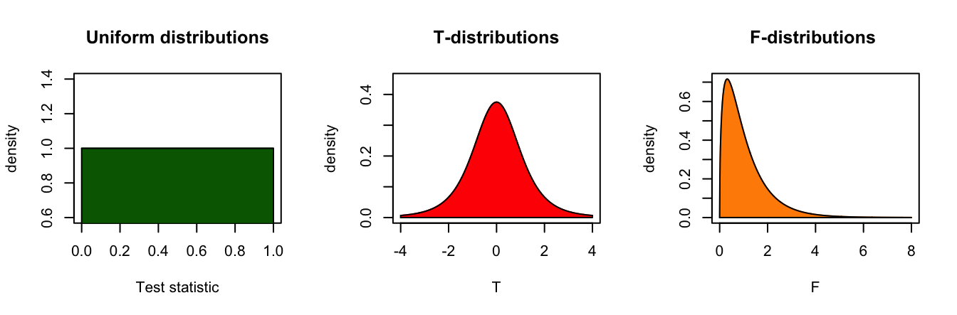
For all continuous probability distributions:
- Total area is always 1
- The probability of one specific test statistic is 0
- x-axis represents the test statistic
- y-axis represents the probability density
T-distribution
Gosset

In probability and statistics, Student’s t-distribution (or simply the t-distribution) is any member of a family of continuous probability distributions that arises when estimating the mean of a normally distributed population in situations where the sample size is small and population standard deviation is unknown.
In the English-language literature it takes its name from William Sealy Gosset’s 1908 paper in Biometrika under the pseudonym “Student”. Gosset worked at the Guinness Brewery in Dublin, Ireland, and was interested in the problems of small samples, for example the chemical properties of barley where sample sizes might be as low as 3 (Wikipedia, 2024).

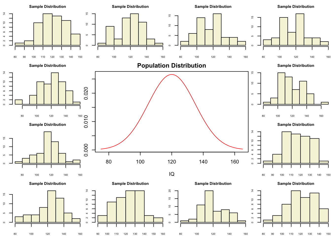
Population distribution
layout(matrix(c(2:6,1,1,7:8,1,1,9:13), 4, 4))

n  = 56    # Sample size
df = n - 1 # Degrees of freedom

mu    = 120
sigma = 15

IQ = seq(mu-45, mu+45, 1)

par(mar=c(4,2,2,0))
plot(IQ, dnorm(IQ, mean = mu, sd = sigma), type='l', col="red", main = "Population Distribution")

n.samples = 12

for(i in 1:n.samples) {

  par(mar=c(2,2,2,0))
  hist(rnorm(n, mu, sigma), main="Sample Distribution", cex.axis=.5, col="beige", cex.main = .75)

}
One sample
Let’s take a larger sample from our normal population.
x = rnorm(n, mu, sigma); x [1] 114.52691 86.89331 140.49631 127.22241 142.18366 132.67762 144.00098
[8] 128.13219 114.62186 114.93952 127.68670 133.69153 145.42975 99.81731
[15] 128.15723 135.29568 172.17921 107.12571 125.85616 111.03657 111.46179
[22] 91.09461 131.81436 128.54418 131.99566 123.69294 105.98591 118.13198
[29] 124.52382 120.40813 112.57450 134.36061 124.81365 106.67286 119.25926
[36] 150.82913 109.40152 119.63508 122.63536 110.49121 103.21775 146.15067
[43] 142.31595 121.71781 113.96224 120.82194 115.19581 137.59349 122.65736
[50] 107.78635 117.41116 114.85585 115.87609 132.15398 143.83374 123.72705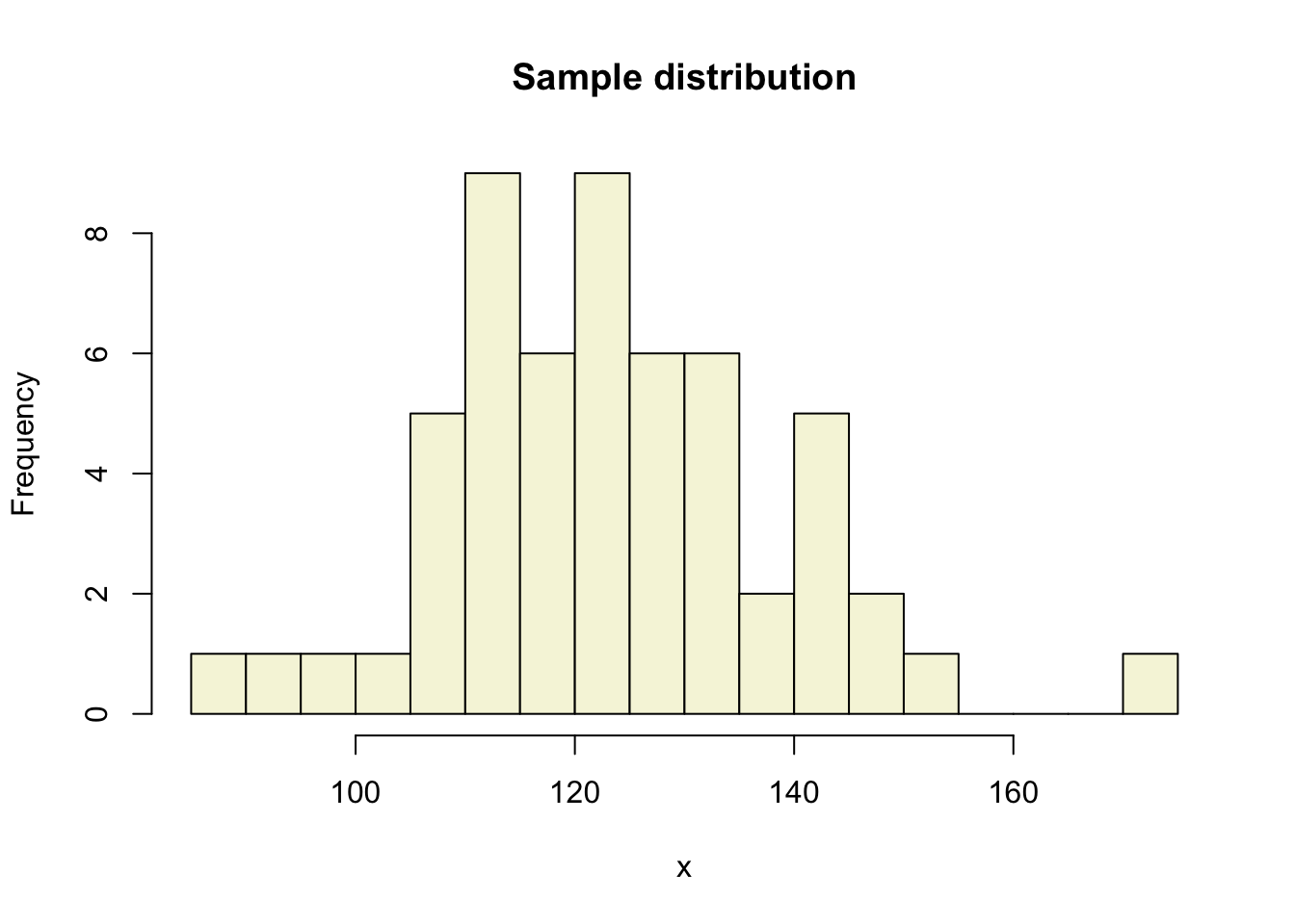
More samples
let’s take more samples.
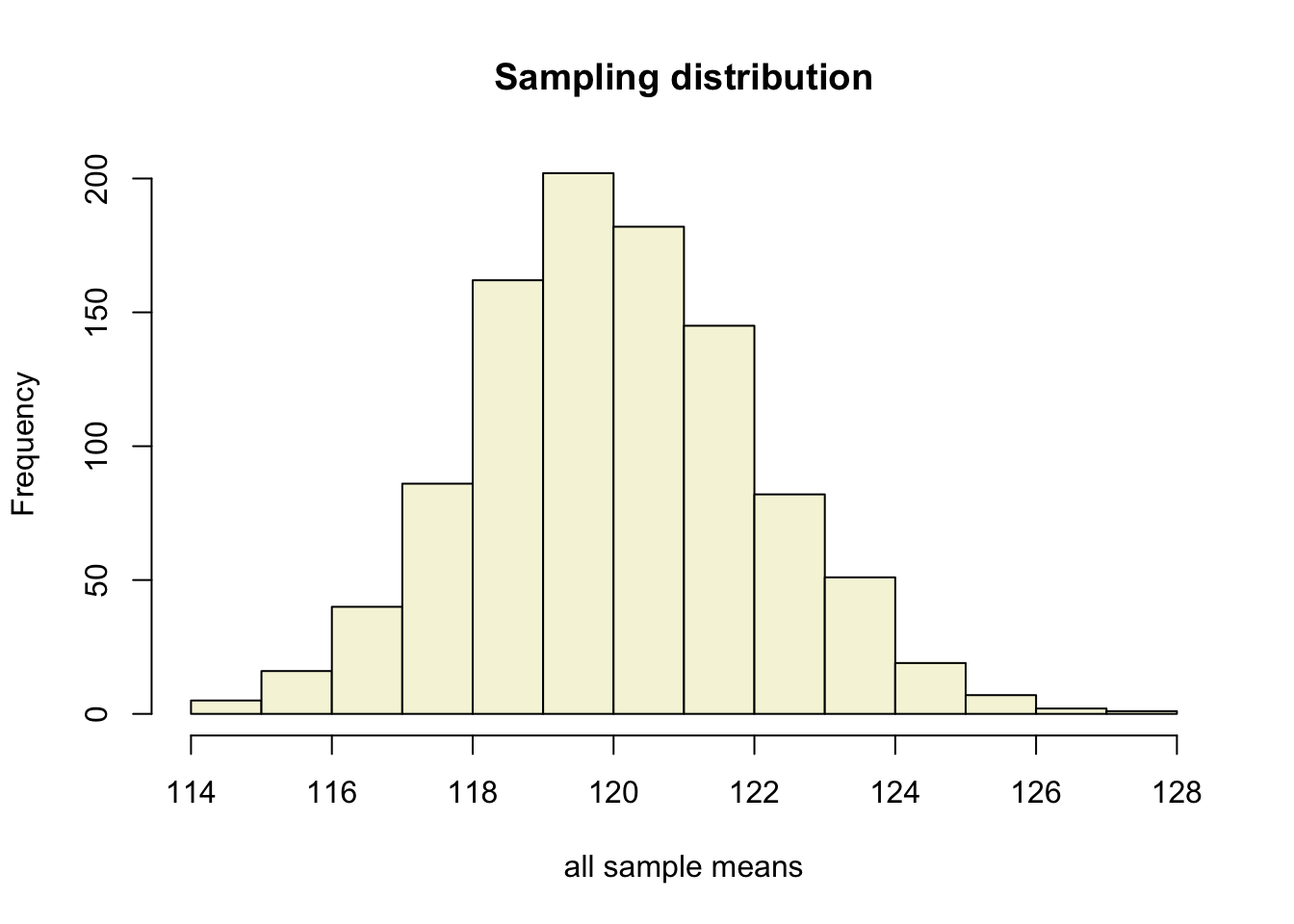
Mean and SE for all samples
     mean.x.values se.x.values
[1,]      119.0084    2.108099
[2,]      122.1465    1.806664
[3,]      120.2006    1.891465
[4,]      120.2139    2.122075
[5,]      119.3888    2.309607
[6,]      122.1463    2.118392
mean.x.values se.x.values
[995,] 119.1899 1.642606
[996,] 122.4428 2.016557
[997,] 122.8243 1.876661
[998,] 119.7023 1.964921
[999,] 117.9064 2.220974
[1000,] 122.3652 1.822761Sampling distribution
of the mean
T-statistic
\[T_{n-1} = \frac{\bar{x}-\mu}{SE_x} = \frac{\bar{x}-\mu}{s_x / \sqrt{n}}\]
So the t-statistic represents the deviation of the sample mean \(\bar{x}\) from the population mean \(\mu\), considering the sample size, expressed as the degrees of freedom \(df = n - 1\)
T-value
\[T_{n-1} = \frac{\bar{x}-\mu}{SE_x} = \frac{\bar{x}-\mu}{s_x / \sqrt{n}}\]
t = (mean(x) - mu) / (sd(x) / sqrt(n))
t
[1] 1.297564Calculate t-values
\[T_{n-1} = \frac{\bar{x}-\mu}{SE_x} = \frac{\bar{x}-\mu}{s_x / \sqrt{n}}\]
t.values = (mean.x.values - mu) / se.x.values mean.x.values mu se.x.values t.values
[995,] 119.1899 120 1.642606 -0.4932032
[996,] 122.4428 120 2.016557 1.2113514
[997,] 122.8243 120 1.876661 1.5049822
[998,] 119.7023 120 1.964921 -0.1515153
[999,] 117.9064 120 2.220974 -0.9426702
[1000,] 122.3652 120 1.822761 1.2975644Sampling distribution t-values
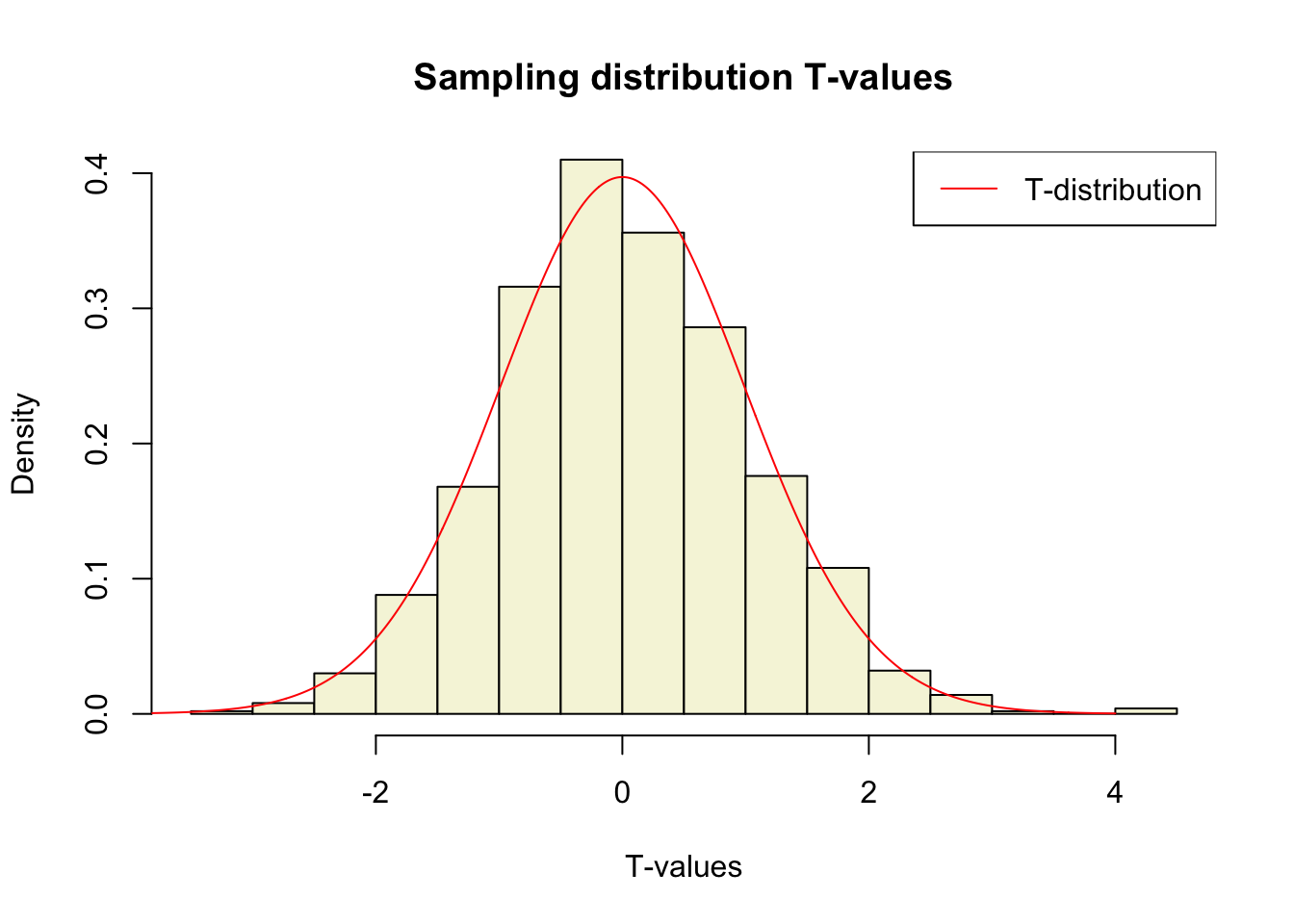
The t-distribution approximates the sampling distribution, hence the name theoretical approximation.
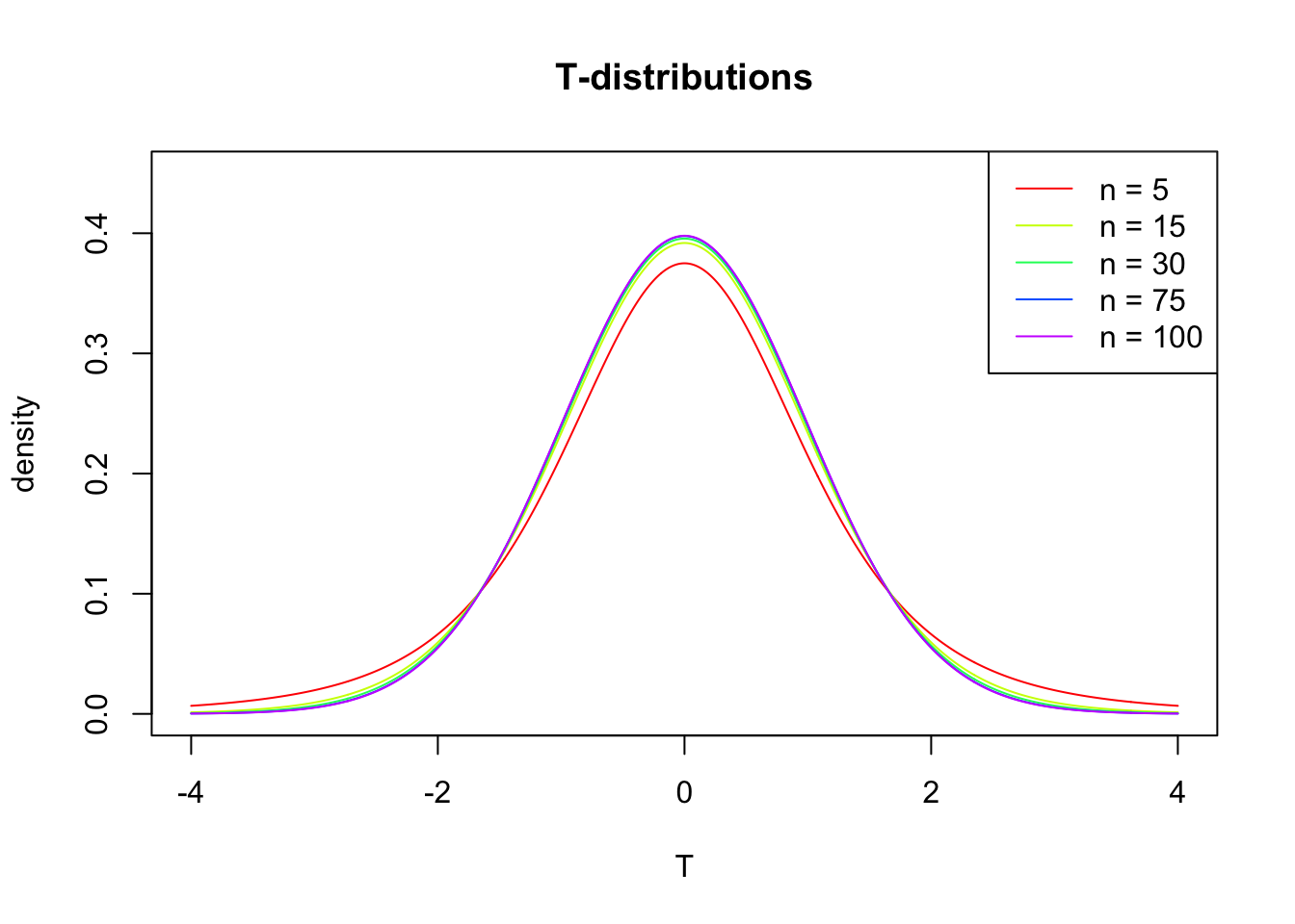
T-distribution
So if the population is normaly distributed (assumption of normality) the t-distribution represents the deviation of sample means from the population mean (\(\mu\)), given a certain sample size (\(df = n - 1\)).
The t-distibution therefore is different for different sample sizes and converges to a standard normal distribution if sample size is large enough.
The t-distribution is defined by the probability density function (PDF):
\[\textstyle\frac{\Gamma \left(\frac{\nu+1}{2} \right)} {\sqrt{\nu\pi}\,\Gamma \left(\frac{\nu}{2} \right)} \left(1+\frac{x^2}{\nu} \right)^{-\frac{\nu+1}{2}}\!\]
where \(\nu\) is the number of degrees of freedom and \(\Gamma\) is the gamma function (Wikipedia, 2024).
Warning
Formula not exam material
End
Contact

References
Wikipedia. (2024). Student’s t-distribution — Wikipedia, the free encyclopedia. http://en.wikipedia.org/w/index.php?title=Student's%20t-distribution&oldid=1202978121.
- Distribution illustration generated with DALL-E by OpenAI