Probability Models
2025-09-08
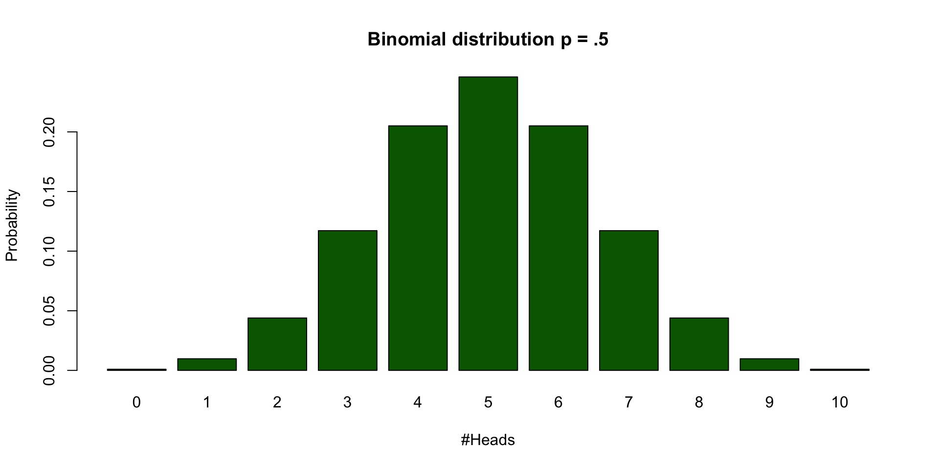
Binomial distribution
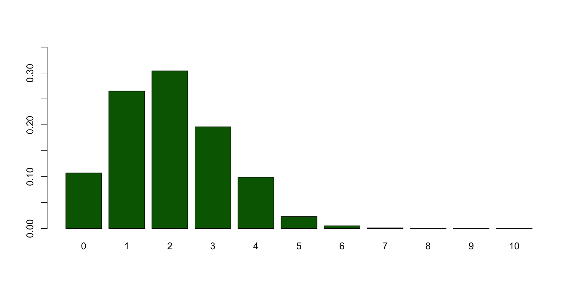
Bootstrapped sampling distribution
Continuous Probability distirbutions
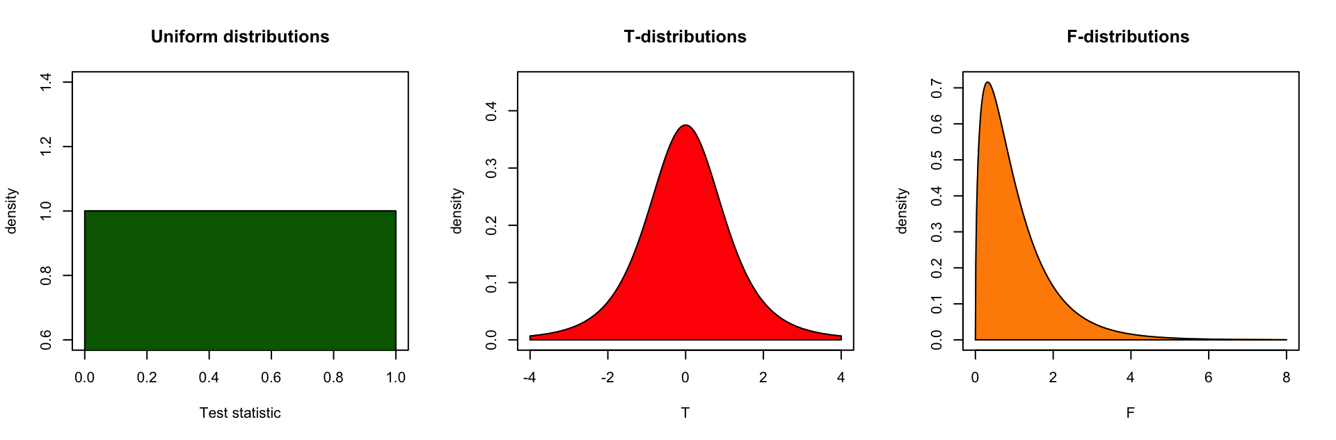
For all continuous probability distributions:
- Total area is always 1
- The probability of one specific test statistic is 0
- x-axis represents the test statistic
- y-axis represents the probability density
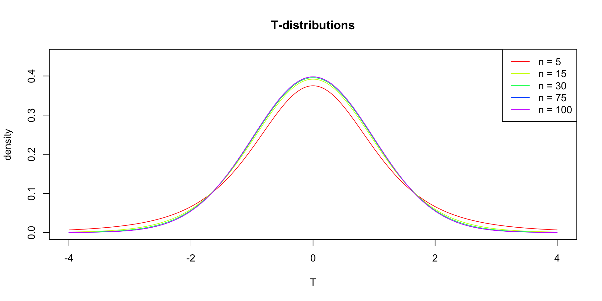
Gosset

In probability and statistics, Student’s t-distribution (or simply the t-distribution) is any member of a family of continuous probability distributions that arises when estimating the mean of a normally distributed population in situations where the sample size is small and population standard deviation is unknown.
In the English-language literature it takes its name from William Sealy Gosset’s 1908 paper in Biometrika under the pseudonym “Student”. Gosset worked at the Guinness Brewery in Dublin, Ireland, and was interested in the problems of small samples, for example the chemical properties of barley where sample sizes might be as low as 3 (Wikipedia, 2024).

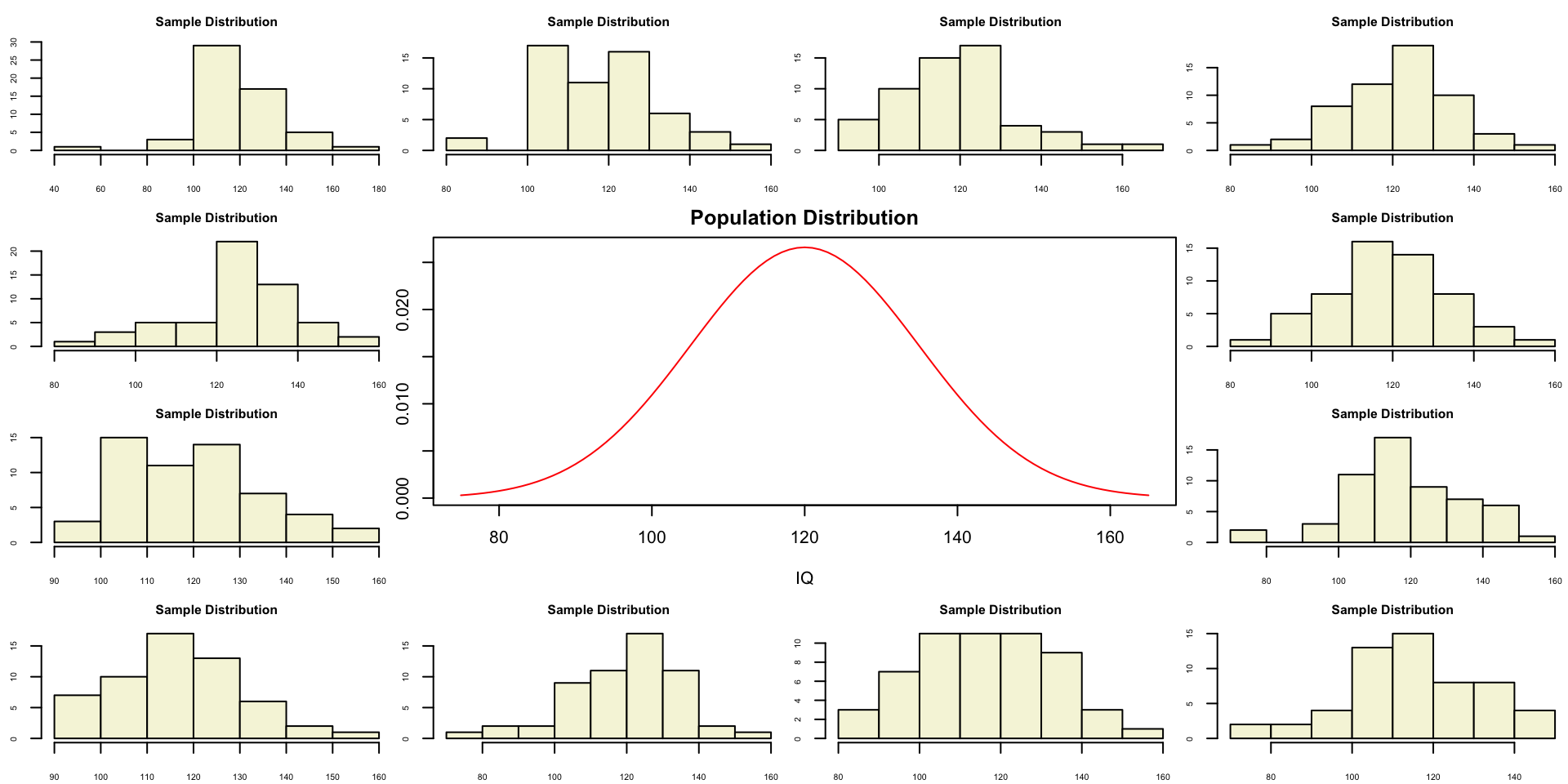
Population distribution
One sample
Let’s take a larger sample from our normal population.
 [1] 125.38159 131.87150  97.91258 106.65761 128.79834 130.37589 104.12035
 [8] 137.92415 135.05426 136.38486 143.56131 110.19591 111.06758  81.15490
[15] 124.67001 137.63382 115.79382 131.16588 122.68704 124.44491 121.53545
[22] 134.25584 121.45674 132.00408 139.55906  98.17081 121.98904 122.04234
[29] 118.85838 136.76335 142.98176 107.43160 115.22124 137.70291 131.19283
[36] 105.44568 131.72974 107.19139 130.45036 116.90866 115.49826 123.98368
[43] 120.42300 114.66301 114.37692 116.56588 112.17237 102.97537 130.09115
[50] 137.89815 104.97558 150.87956  95.52687 143.39545 114.49853 121.09488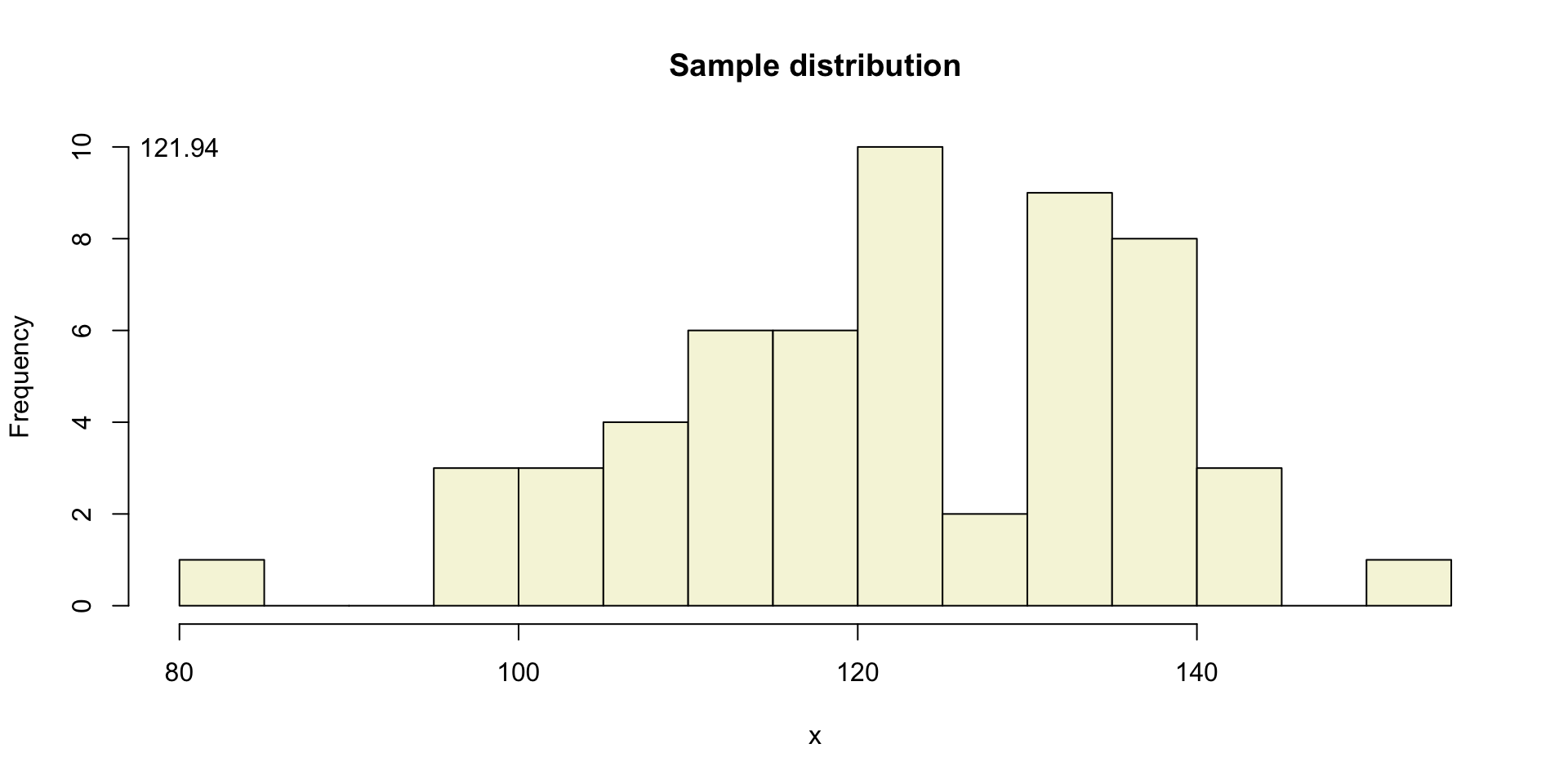
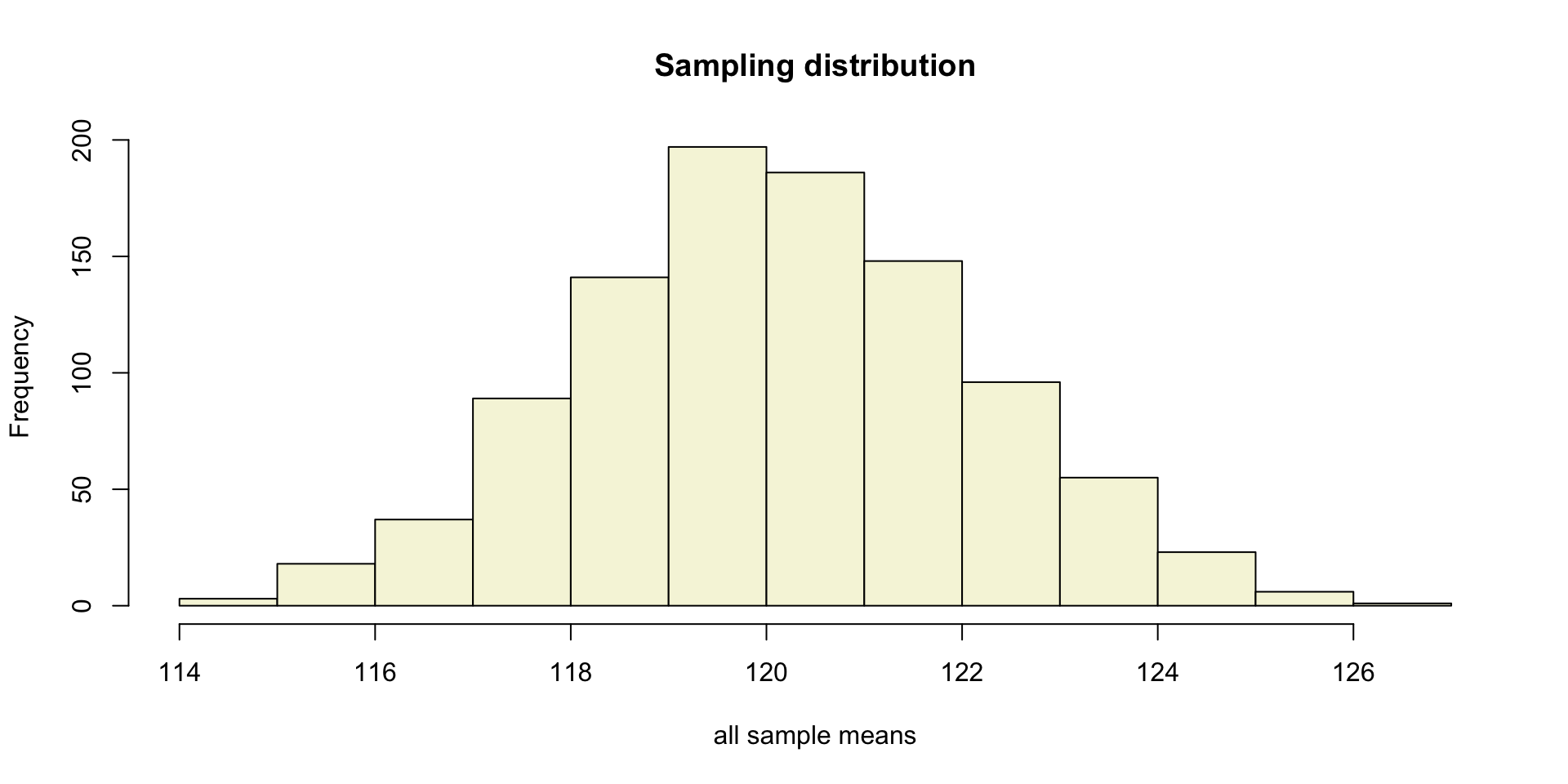
Sampling distribution
of the mean
Sampling distribution t-values
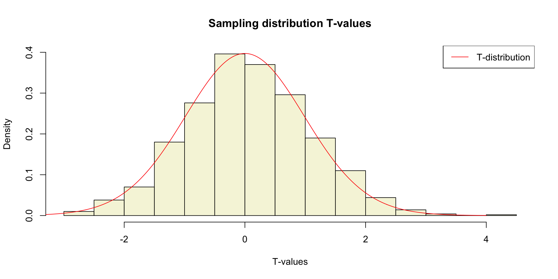
The t-distribution approximates the sampling distribution, hence the name theoretical approximation.
Contact
