  Toss1 Toss2
1     0     0
2     1     0
3     0     1
4 1 1Probability Models
Why do we need them
Exact approach
Coin values
Lets start simple and throw only 2 times with a fair coin. Assigning 1 for heads and 0 for tails.
The coin can only have the values 0, 1, heads or tails.
Permutation
If we throw 2 times we have the following possible outcomes.
Number of heads
With frequency of heads being
  Toss1 Toss2 frequency
1     0     0         0
2     1     0         1
3     0     1         1
4     1     1         2
Probabilities
For each coin toss, disregarding the outcom, there is a .5 probability of landing heads.
  Toss1 Toss2
1   0.5   0.5
2   0.5   0.5
3   0.5   0.5
4   0.5   0.5
So for each we can specify the total probability by applying the product rule (e.g. multiplying the probabilities)
  Toss1 Toss2 probability
1   0.5   0.5        0.25
2   0.5   0.5        0.25
3   0.5   0.5        0.25
4   0.5   0.5        0.25
Which is the same for all outcomes.
Discrete probabilities
Though some outcomes occurs more often. Throwing 0 times heads, only occurs once and hence has a probability of .25. But throwing 1 times heads, can occur in two situations. So, for this situation we can add up the probabilities.
  Toss1 Toss2 frequency probability
1     0     0         0        0.25
2     1     0         1        0.25
3     0     1         1        0.25
4     1     1         2        0.25
Frequecy and probability distribution
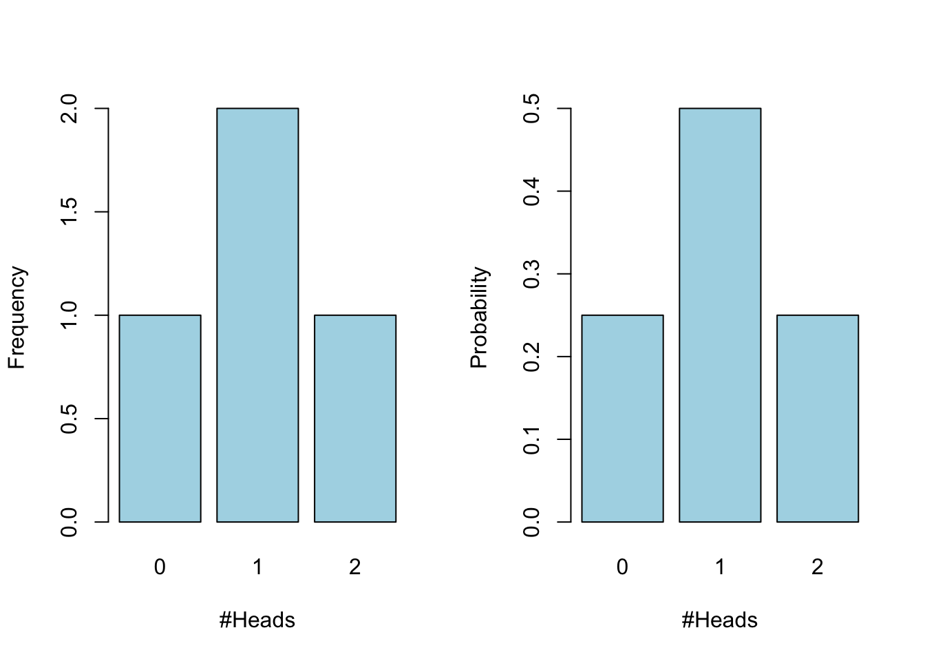
10 tosses
| Toss1 | Toss2 | Toss3 | Toss4 | Toss5 | Toss6 | Toss7 | Toss8 | Toss9 | Toss10 |
|---|---|---|---|---|---|---|---|---|---|
| 0.5 | 0.5 | 0.5 | 0.5 | 0.5 | 0.5 | 0.5 | 0.5 | 0.5 | 0.5 |
| 0.5 | 0.5 | 0.5 | 0.5 | 0.5 | 0.5 | 0.5 | 0.5 | 0.5 | 0.5 |
| 0.5 | 0.5 | 0.5 | 0.5 | 0.5 | 0.5 | 0.5 | 0.5 | 0.5 | 0.5 |
| 0.5 | 0.5 | 0.5 | 0.5 | 0.5 | 0.5 | 0.5 | 0.5 | 0.5 | 0.5 |
| 0.5 | 0.5 | 0.5 | 0.5 | 0.5 | 0.5 | 0.5 | 0.5 | 0.5 | 0.5 |
| 0.5 | 0.5 | 0.5 | 0.5 | 0.5 | 0.5 | 0.5 | 0.5 | 0.5 | 0.5 |
| 0.5 | 0.5 | 0.5 | 0.5 | 0.5 | 0.5 | 0.5 | 0.5 | 0.5 | 0.5 |
| Toss1 | Toss2 | Toss3 | Toss4 | Toss5 | Toss6 | Toss7 | Toss8 | Toss9 | Toss10 | probability |
|---|---|---|---|---|---|---|---|---|---|---|
| 0.5 | 0.5 | 0.5 | 0.5 | 0.5 | 0.5 | 0.5 | 0.5 | 0.5 | 0.5 | 0.0009766 |
| 0.5 | 0.5 | 0.5 | 0.5 | 0.5 | 0.5 | 0.5 | 0.5 | 0.5 | 0.5 | 0.0009766 |
| 0.5 | 0.5 | 0.5 | 0.5 | 0.5 | 0.5 | 0.5 | 0.5 | 0.5 | 0.5 | 0.0009766 |
| 0.5 | 0.5 | 0.5 | 0.5 | 0.5 | 0.5 | 0.5 | 0.5 | 0.5 | 0.5 | 0.0009766 |
| 0.5 | 0.5 | 0.5 | 0.5 | 0.5 | 0.5 | 0.5 | 0.5 | 0.5 | 0.5 | 0.0009766 |
| #Heads | frequencies | Probabilities |
|---|---|---|
| 0 | 1 | 0.0009766 |
| 1 | 10 | 0.0097656 |
| 2 | 45 | 0.0439453 |
| 3 | 120 | 0.1171875 |
| 4 | 210 | 0.2050781 |
| 5 | 252 | 0.2460938 |
| 6 | 210 | 0.2050781 |
| 7 | 120 | 0.1171875 |
| 8 | 45 | 0.0439453 |
| 9 | 10 | 0.0097656 |
| 10 | 1 | 0.0009766 |
Binomial distribution
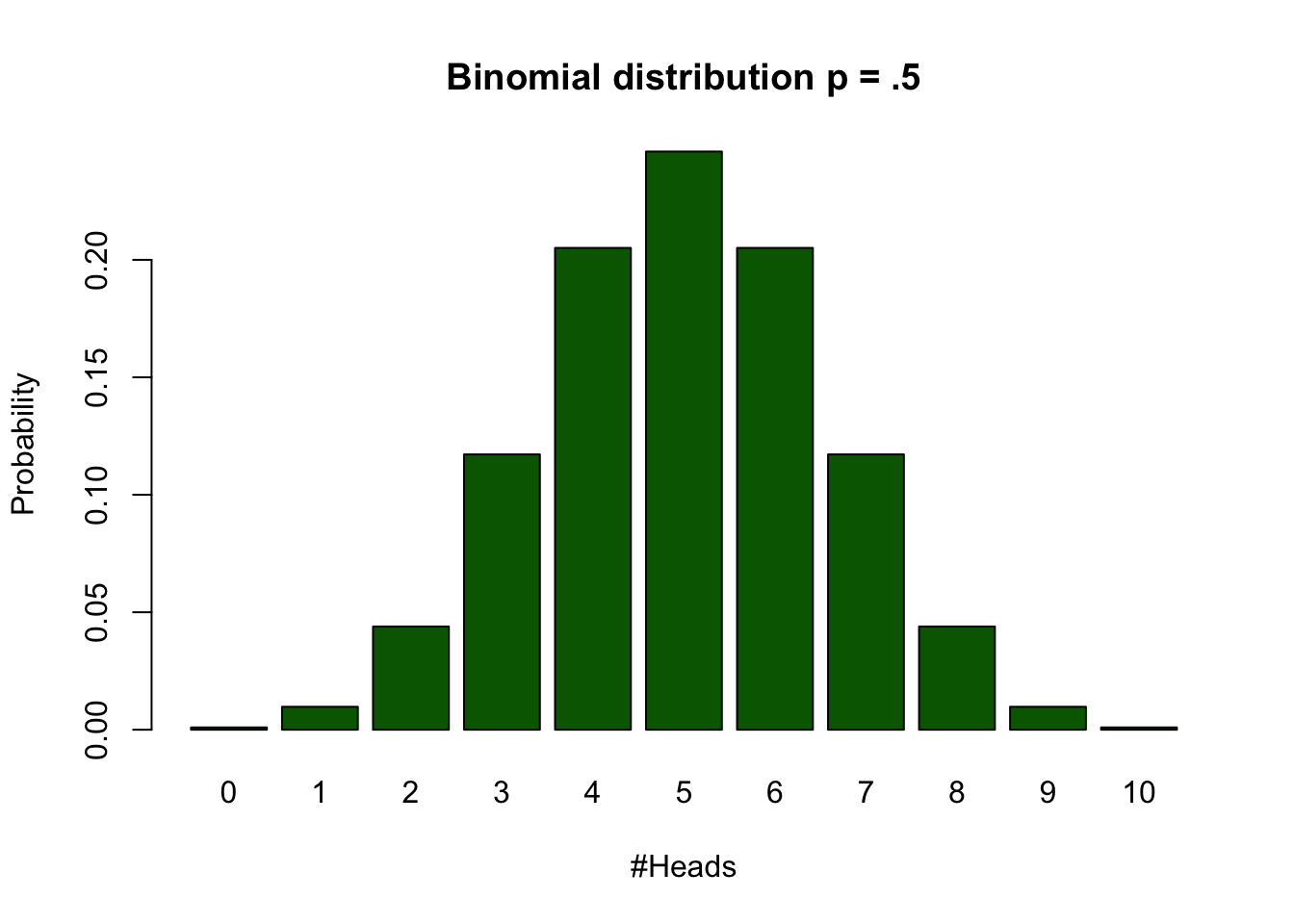
Calculate binomial probabilities
\[ {n\choose k}p^k(1-p)^{n-k}, \small {n\choose k} = \frac{n!}{k!(n-k)!} \]
n = 10   # Sample size
k = 0:10 # Discrete probability space
p = .5 # Probability of head| n | k | p | n! | k! | (n-k)! | (n over k) | p^k | (1-p)^(n-k) | Binom Prob |
|---|---|---|---|---|---|---|---|---|---|
| 10 | 0 | 0.5 | 3628800 | 1 | 3628800 | 1 | 1.0000000 | 0.0009766 | 0.0009766 |
| 10 | 1 | 0.5 | 3628800 | 1 | 362880 | 10 | 0.5000000 | 0.0019531 | 0.0097656 |
| 10 | 2 | 0.5 | 3628800 | 2 | 40320 | 45 | 0.2500000 | 0.0039063 | 0.0439453 |
| 10 | 3 | 0.5 | 3628800 | 6 | 5040 | 120 | 0.1250000 | 0.0078125 | 0.1171875 |
| 10 | 4 | 0.5 | 3628800 | 24 | 720 | 210 | 0.0625000 | 0.0156250 | 0.2050781 |
| 10 | 5 | 0.5 | 3628800 | 120 | 120 | 252 | 0.0312500 | 0.0312500 | 0.2460938 |
| 10 | 6 | 0.5 | 3628800 | 720 | 24 | 210 | 0.0156250 | 0.0625000 | 0.2050781 |
| 10 | 7 | 0.5 | 3628800 | 5040 | 6 | 120 | 0.0078125 | 0.1250000 | 0.1171875 |
| 10 | 8 | 0.5 | 3628800 | 40320 | 2 | 45 | 0.0039063 | 0.2500000 | 0.0439453 |
| 10 | 9 | 0.5 | 3628800 | 362880 | 1 | 10 | 0.0019531 | 0.5000000 | 0.0097656 |
| 10 | 10 | 0.5 | 3628800 | 3628800 | 1 | 1 | 0.0009766 | 1.0000000 | 0.0009766 |
Formula not exam material
Bootstrapping
Sampling from your sample to approximate the sampling distribution.
My Coin tosses
my.tosses = c(1,0,0,0,0,1,0,0,0,0)Sample from the sample
Sampling with replacement
sample(my.tosses, replace = TRUE) [1] 0 0 0 1 0 1 0 0 1 0sample(my.tosses, replace = TRUE) [1] 0 1 1 0 0 1 0 0 0 1sample(my.tosses, replace = TRUE) [1] 0 0 0 0 0 0 0 0 0 1sample(my.tosses, replace = TRUE) [1] 0 0 0 0 0 0 0 0 0 0Sampling from the sample
n.samples = 1000
n.heads = vector()

for (i in 1:n.samples) {
  my.sample <- sample(my.tosses, replace = TRUE)

  n.heads[i] <- sum(my.sample)
}| 1 | 0 | 1 | 0 | 2 | 0 | 1 | 1 | 1 | 1 | 2 | 1 | 0 | 3 | 0 | 3 | 1 | 2 | 3 | 3 | 4 | 1 | 5 | 0 | 2 | 1 | 1 | 2 | 4 | 2 | 0 | 1 | 1 | 3 | 2 | 4 | 1 | 2 | 2 | 2 |
| 1 | 0 | 1 | 2 | 2 | 2 | 1 | 2 | 1 | 3 | 0 | 3 | 3 | 1 | 3 | 1 | 0 | 0 | 0 | 2 | 0 | 1 | 3 | 5 | 0 | 2 | 0 | 4 | 2 | 1 | 0 | 1 | 5 | 2 | 3 | 1 | 3 | 3 | 1 | 1 |
| 4 | 2 | 1 | 0 | 1 | 0 | 2 | 0 | 3 | 3 | 4 | 3 | 3 | 2 | 1 | 1 | 3 | 1 | 3 | 3 | 3 | 2 | 2 | 2 | 0 | 0 | 3 | 2 | 3 | 2 | 2 | 2 | 2 | 1 | 2 | 3 | 5 | 2 | 2 | 2 |
| 3 | 3 | 3 | 5 | 1 | 4 | 2 | 3 | 1 | 2 | 2 | 4 | 1 | 3 | 2 | 1 | 5 | 2 | 1 | 1 | 1 | 4 | 1 | 3 | 1 | 5 | 0 | 1 | 3 | 2 | 2 | 1 | 2 | 1 | 2 | 0 | 0 | 2 | 2 | 2 |
| 2 | 4 | 2 | 4 | 3 | 1 | 2 | 2 | 0 | 2 | 1 | 1 | 0 | 3 | 3 | 2 | 3 | 3 | 3 | 2 | 2 | 1 | 1 | 1 | 0 | 1 | 0 | 3 | 1 | 1 | 3 | 1 | 3 | 3 | 3 | 0 | 3 | 3 | 2 | 0 |
| 0 | 2 | 3 | 0 | 1 | 0 | 0 | 2 | 2 | 2 | 1 | 2 | 1 | 0 | 2 | 1 | 2 | 1 | 2 | 1 | 3 | 4 | 4 | 3 | 2 | 3 | 2 | 4 | 1 | 2 | 1 | 1 | 2 | 1 | 1 | 3 | 2 | 1 | 2 | 0 |
| 3 | 2 | 2 | 2 | 2 | 5 | 3 | 2 | 3 | 2 | 4 | 0 | 1 | 2 | 3 | 1 | 4 | 0 | 2 | 1 | 3 | 1 | 1 | 3 | 2 | 2 | 1 | 4 | 0 | 2 | 0 | 2 | 2 | 1 | 0 | 4 | 5 | 1 | 1 | 3 |
| 1 | 2 | 1 | 2 | 3 | 2 | 5 | 2 | 2 | 3 | 1 | 3 | 4 | 3 | 2 | 0 | 2 | 2 | 3 | 1 | 1 | 2 | 2 | 1 | 2 | 5 | 0 | 3 | 2 | 5 | 3 | 4 | 1 | 3 | 0 | 0 | 3 | 3 | 2 | 2 |
| 0 | 1 | 2 | 2 | 1 | 0 | 2 | 2 | 2 | 2 | 2 | 1 | 2 | 2 | 1 | 2 | 4 | 0 | 2 | 2 | 3 | 1 | 1 | 1 | 1 | 2 | 2 | 1 | 2 | 2 | 1 | 1 | 2 | 3 | 1 | 2 | 3 | 2 | 2 | 2 |
| 2 | 2 | 1 | 2 | 5 | 1 | 2 | 1 | 1 | 2 | 2 | 2 | 2 | 4 | 1 | 1 | 2 | 2 | 3 | 1 | 4 | 6 | 3 | 1 | 2 | 2 | 3 | 0 | 1 | 2 | 2 | 2 | 2 | 2 | 1 | 2 | 4 | 2 | 4 | 2 |
| 6 | 3 | 2 | 3 | 2 | 0 | 2 | 1 | 1 | 1 | 3 | 3 | 2 | 3 | 8 | 6 | 6 | 4 | 2 | 1 | 2 | 1 | 1 | 1 | 1 | 2 | 2 | 2 | 1 | 2 | 7 | 3 | 0 | 2 | 3 | 1 | 2 | 1 | 4 | 2 |
| 3 | 1 | 4 | 2 | 2 | 3 | 1 | 2 | 1 | 1 | 3 | 2 | 2 | 1 | 0 | 2 | 1 | 1 | 3 | 5 | 2 | 0 | 1 | 2 | 3 | 3 | 2 | 4 | 3 | 1 | 1 | 1 | 1 | 4 | 0 | 2 | 2 | 2 | 3 | 3 |
| 1 | 7 | 1 | 2 | 3 | 2 | 3 | 1 | 3 | 3 | 1 | 1 | 3 | 4 | 1 | 2 | 2 | 1 | 3 | 3 | 2 | 2 | 1 | 1 | 3 | 4 | 1 | 5 | 3 | 3 | 4 | 2 | 2 | 1 | 2 | 3 | 2 | 2 | 2 | 2 |
| 2 | 2 | 0 | 0 | 1 | 1 | 4 | 2 | 1 | 4 | 3 | 3 | 2 | 2 | 1 | 1 | 2 | 3 | 2 | 3 | 4 | 4 | 2 | 1 | 1 | 2 | 0 | 0 | 2 | 2 | 4 | 2 | 3 | 2 | 1 | 2 | 1 | 1 | 2 | 2 |
| 2 | 2 | 1 | 0 | 2 | 0 | 3 | 1 | 2 | 1 | 4 | 1 | 1 | 3 | 2 | 3 | 0 | 1 | 0 | 1 | 3 | 3 | 3 | 3 | 3 | 1 | 0 | 4 | 1 | 2 | 3 | 1 | 4 | 2 | 1 | 3 | 2 | 2 | 4 | 3 |
| 4 | 1 | 2 | 1 | 0 | 0 | 2 | 4 | 4 | 3 | 1 | 4 | 1 | 4 | 1 | 1 | 3 | 4 | 2 | 4 | 2 | 1 | 3 | 2 | 2 | 1 | 0 | 0 | 1 | 1 | 4 | 4 | 1 | 1 | 0 | 3 | 4 | 1 | 0 | 3 |
| 0 | 0 | 2 | 0 | 2 | 2 | 1 | 4 | 4 | 3 | 2 | 3 | 3 | 3 | 2 | 4 | 0 | 4 | 3 | 6 | 2 | 6 | 2 | 1 | 1 | 2 | 2 | 4 | 1 | 1 | 1 | 2 | 2 | 1 | 1 | 1 | 4 | 0 | 1 | 0 |
| 2 | 3 | 3 | 2 | 2 | 2 | 3 | 2 | 2 | 1 | 4 | 1 | 1 | 0 | 3 | 3 | 1 | 2 | 2 | 2 | 3 | 3 | 1 | 3 | 2 | 1 | 3 | 1 | 2 | 2 | 2 | 3 | 0 | 4 | 2 | 1 | 2 | 1 | 2 | 3 |
| 3 | 2 | 0 | 1 | 1 | 0 | 3 | 1 | 2 | 1 | 1 | 0 | 4 | 1 | 1 | 2 | 3 | 3 | 6 | 1 | 2 | 3 | 1 | 3 | 1 | 2 | 3 | 1 | 1 | 3 | 3 | 0 | 0 | 1 | 3 | 2 | 0 | 2 | 3 | 3 |
| 3 | 2 | 4 | 3 | 0 | 2 | 1 | 2 | 1 | 2 | 0 | 1 | 1 | 5 | 0 | 1 | 3 | 5 | 2 | 3 | 4 | 0 | 1 | 3 | 2 | 1 | 2 | 1 | 3 | 0 | 0 | 1 | 6 | 2 | 4 | 4 | 0 | 2 | 3 | 2 |
| 3 | 4 | 2 | 2 | 1 | 0 | 1 | 2 | 1 | 4 | 1 | 0 | 2 | 1 | 4 | 2 | 2 | 3 | 1 | 3 | 2 | 2 | 3 | 2 | 1 | 1 | 3 | 3 | 2 | 0 | 3 | 1 | 1 | 2 | 2 | 4 | 1 | 2 | 2 | 1 |
| 1 | 1 | 1 | 1 | 0 | 2 | 4 | 1 | 3 | 2 | 1 | 3 | 1 | 3 | 5 | 2 | 2 | 1 | 1 | 3 | 3 | 3 | 2 | 2 | 5 | 1 | 3 | 3 | 5 | 1 | 2 | 6 | 3 | 4 | 1 | 1 | 2 | 2 | 5 | 3 |
| 1 | 3 | 1 | 0 | 2 | 3 | 0 | 4 | 2 | 2 | 2 | 1 | 3 | 5 | 1 | 3 | 1 | 3 | 2 | 2 | 1 | 0 | 2 | 1 | 2 | 4 | 2 | 2 | 1 | 0 | 2 | 2 | 2 | 0 | 2 | 1 | 3 | 1 | 4 | 2 |
| 3 | 3 | 1 | 3 | 4 | 2 | 1 | 3 | 3 | 4 | 4 | 2 | 5 | 1 | 3 | 3 | 0 | 2 | 1 | 4 | 0 | 2 | 0 | 5 | 3 | 2 | 4 | 1 | 4 | 3 | 2 | 3 | 4 | 2 | 1 | 1 | 1 | 4 | 3 | 3 |
| 0 | 5 | 1 | 2 | 1 | 1 | 4 | 2 | 0 | 2 | 0 | 3 | 1 | 3 | 1 | 3 | 5 | 2 | 2 | 2 | 0 | 0 | 1 | 2 | 1 | 3 | 1 | 5 | 3 | 2 | 1 | 2 | 1 | 2 | 1 | 0 | 3 | 1 | 1 | 2 |
Frequencies
Frequencies for number of heads per sample.
| 0 | 1 | 2 | 3 | 4 | 5 | 6 | 7 | 8 | 9 | 10 | |
|---|---|---|---|---|---|---|---|---|---|---|---|
| Freq | 108 | 269 | 305 | 196 | 83 | 27 | 9 | 2 | 1 | 0 | 0 |
Bootstrapped sampling distribution
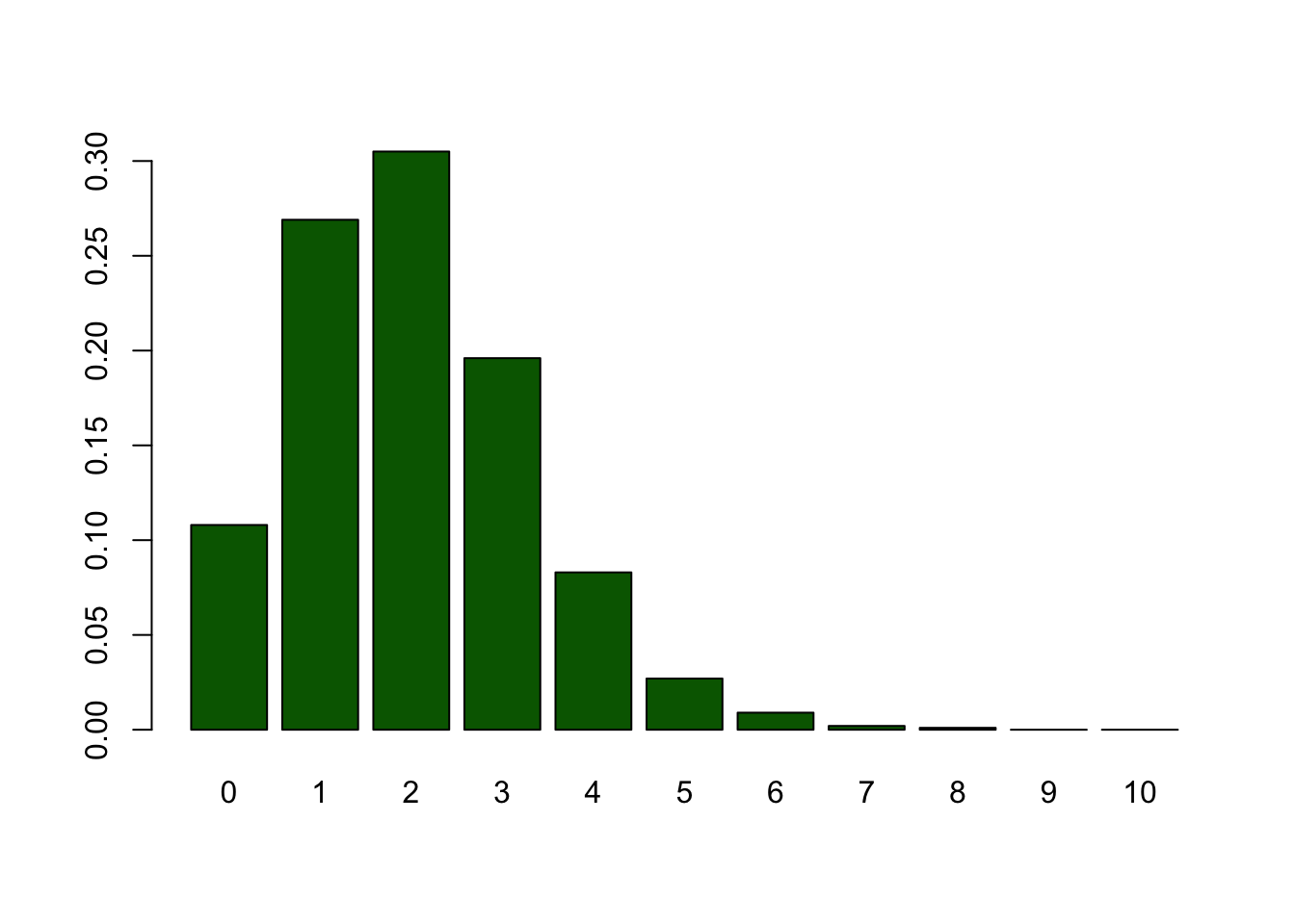
Theoretical Approximations
Continuous Probability distirbutions

For all continuous probability distributions:
- Total area is always 1
- The probability of one specific test statistic is 0
- x-axis represents the test statistic
- y-axis represents the probability density
T-distribution
Gosset

In probability and statistics, Student’s t-distribution (or simply the t-distribution) is any member of a family of continuous probability distributions that arises when estimating the mean of a normally distributed population in situations where the sample size is small and population standard deviation is unknown.
In the English-language literature it takes its name from William Sealy Gosset’s 1908 paper in Biometrika under the pseudonym “Student”. Gosset worked at the Guinness Brewery in Dublin, Ireland, and was interested in the problems of small samples, for example the chemical properties of barley where sample sizes might be as low as 3 (Wikipedia, 2024).
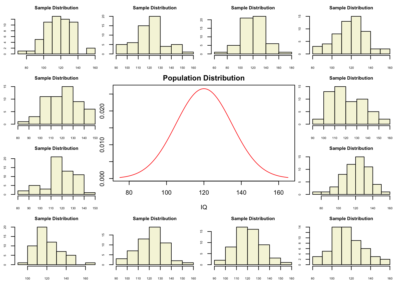
Population distribution
layout(matrix(c(2:6,1,1,7:8,1,1,9:13), 4, 4))

n  = 56    # Sample size
df = n - 1 # Degrees of freedom

mu    = 120
sigma = 15

IQ = seq(mu-45, mu+45, 1)

par(mar=c(4,2,2,0))
plot(IQ, dnorm(IQ, mean = mu, sd = sigma), type='l', col="red", main = "Population Distribution")

n.samples = 12

for(i in 1:n.samples) {

  par(mar=c(2,2,2,0))
  hist(rnorm(n, mu, sigma), main="Sample Distribution", cex.axis=.5, col="beige", cex.main = .75)

}
One sample
Let’s take a larger sample from our normal population.
x = rnorm(n, mu, sigma); x [1] 97.06428 114.31771 103.64482 140.67038 128.99539 117.87526 111.73642
[8] 105.48477 106.31656 129.45169 125.08566 101.88818 115.08274 104.44234
[15] 122.49280 108.79976 127.81236 107.16964 127.74160 110.83698 113.79568
[22] 109.32256 124.79154 129.53559 121.57500 108.01930 136.10072 124.34897
[29] 103.89350 130.34960 97.45505 118.56125 122.91603 106.65062 118.39349
[36] 154.17325 131.21718 117.53183 148.10957 136.79388 121.68563 125.09256
[43] 107.17690 119.11510 132.22669 101.97368 131.40654 75.32125 146.37583
[50] 130.65990 109.58043 130.64950 133.73613 126.37083 107.72237 97.71106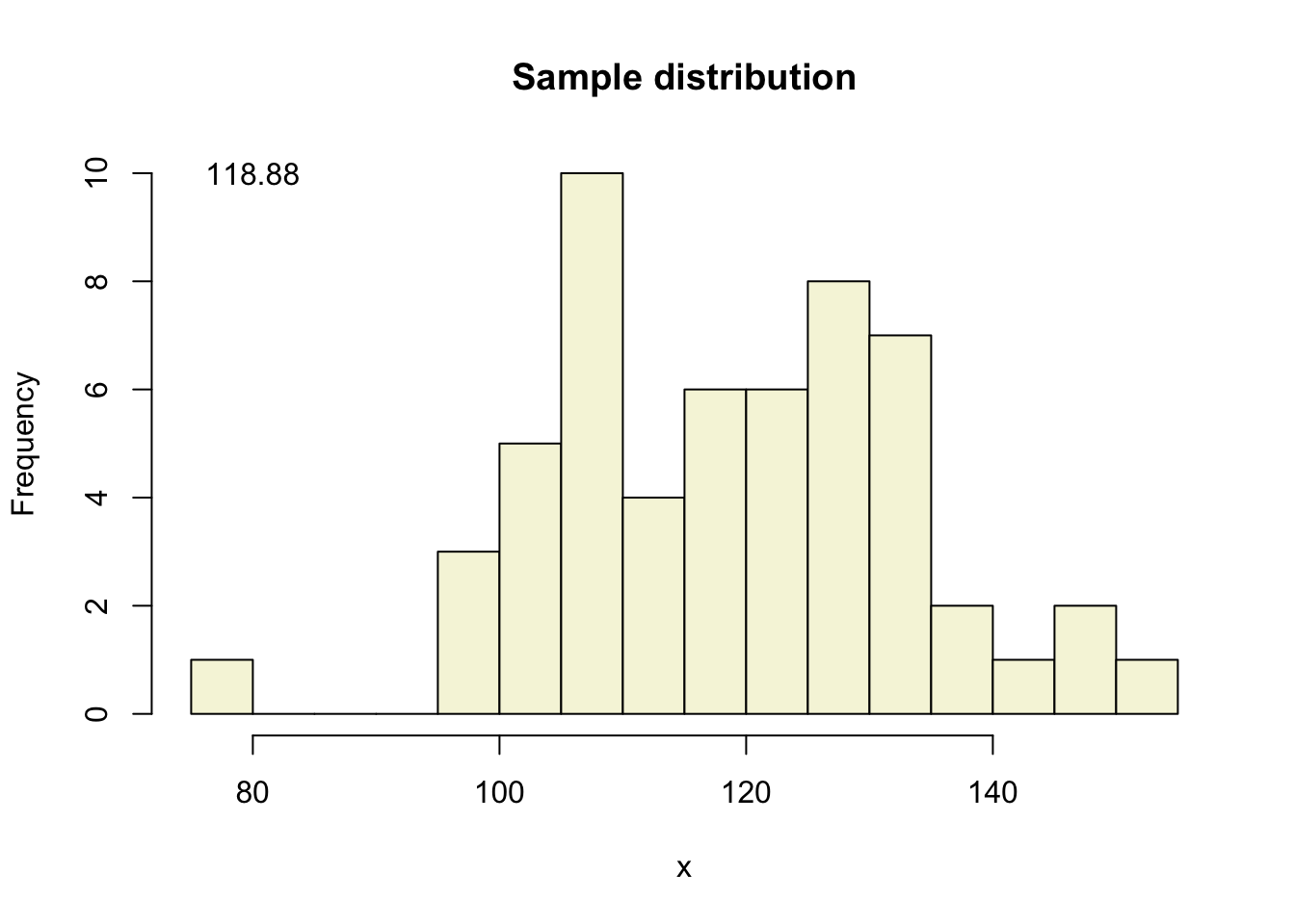
More samples
let’s take more samples.
Mean and SE for all samples
| mean.x.values | se.x.values |
|---|---|
| 118.7716 | 2.134338 |
| 120.4047 | 1.712772 |
| 119.8567 | 1.822675 |
| 119.0746 | 1.986970 |
| 117.9119 | 2.144666 |
| 121.2183 | 1.804641 |
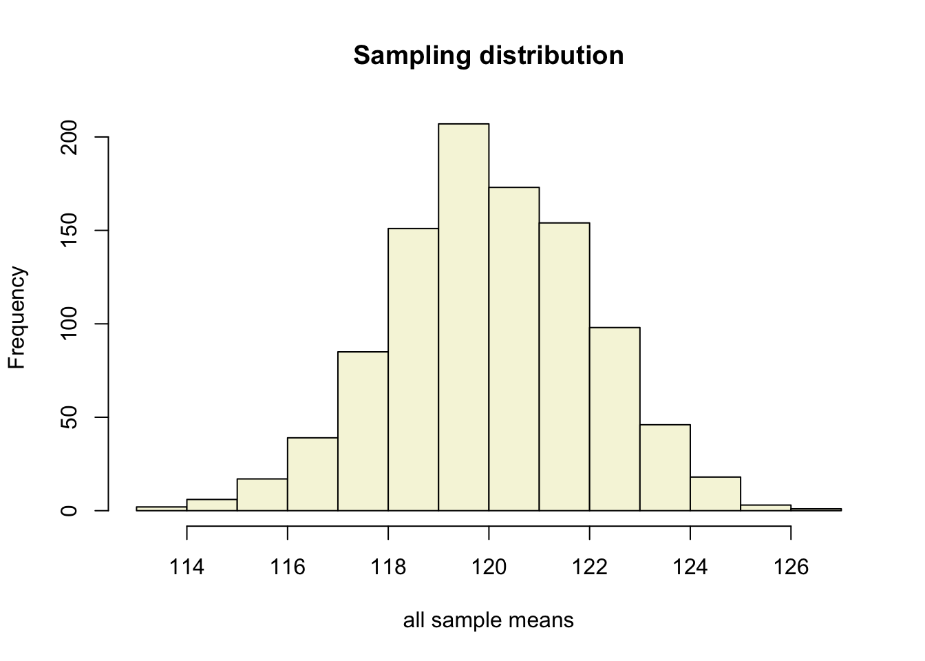
Sampling distribution
of the mean
T-statistic
\[T_{n-1} = \frac{\bar{x}-\mu}{SE_x} = \frac{\bar{x}-\mu}{s_x / \sqrt{n}}\]
So the t-statistic represents the deviation of the sample mean \(\bar{x}\) from the population mean \(\mu\), considering the sample size, expressed as the degrees of freedom \(df = n - 1\)
T-value
\[T_{n-1} = \frac{\bar{x}-\mu}{SE_x} = \frac{\bar{x}-\mu}{s_x / \sqrt{n}}\]
t = (mean(x) - mu) / (sd(x) / sqrt(n))
t
[1] 1.509039Calculate t-values
\[T_{n-1} = \frac{\bar{x}-\mu}{SE_x} = \frac{\bar{x}-\mu}{s_x / \sqrt{n}}\]
t.values = (mean.x.values - mu) / se.x.values mean.x.values mu se.x.values t.values
[995,] 119.9388 120 2.490080 -0.02456887
[996,] 124.0480 120 1.996019 2.02802302
[997,] 118.1232 120 2.214038 -0.84766424
[998,] 120.4651 120 1.882545 0.24704776
[999,] 118.7644 120 1.976912 -0.62499384
[1000,] 123.1174 120 2.065799 1.50903941Sampling distribution t-values
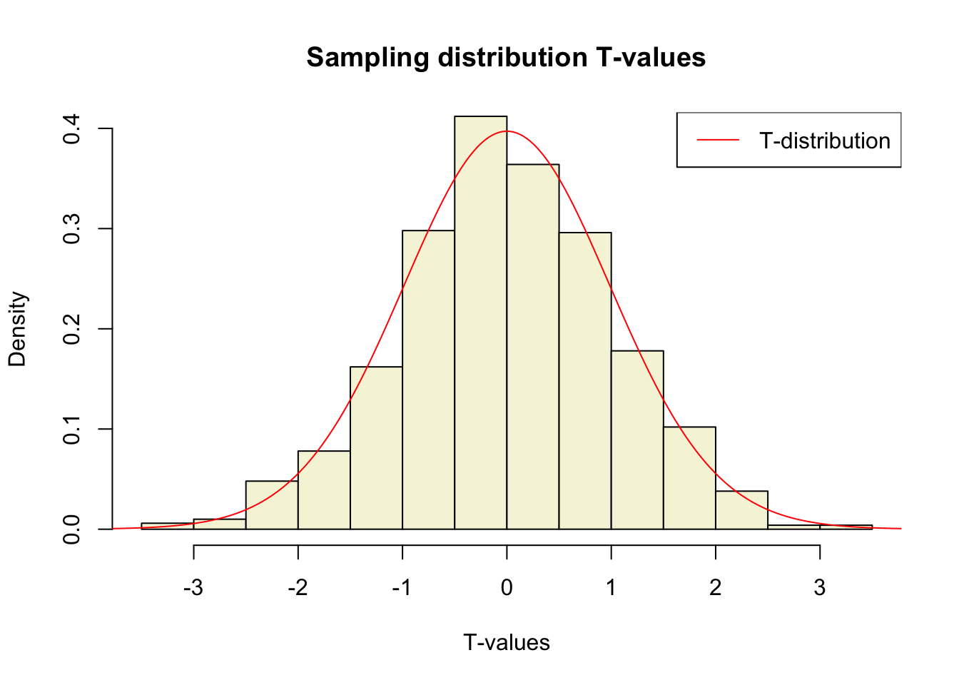
The t-distribution approximates the sampling distribution, hence the name theoretical approximation.
T-distribution
So if the population is normaly distributed (assumption of normality) the t-distribution represents the deviation of sample means from the population mean (\(\mu\)), given a certain sample size (\(df = n - 1\)).
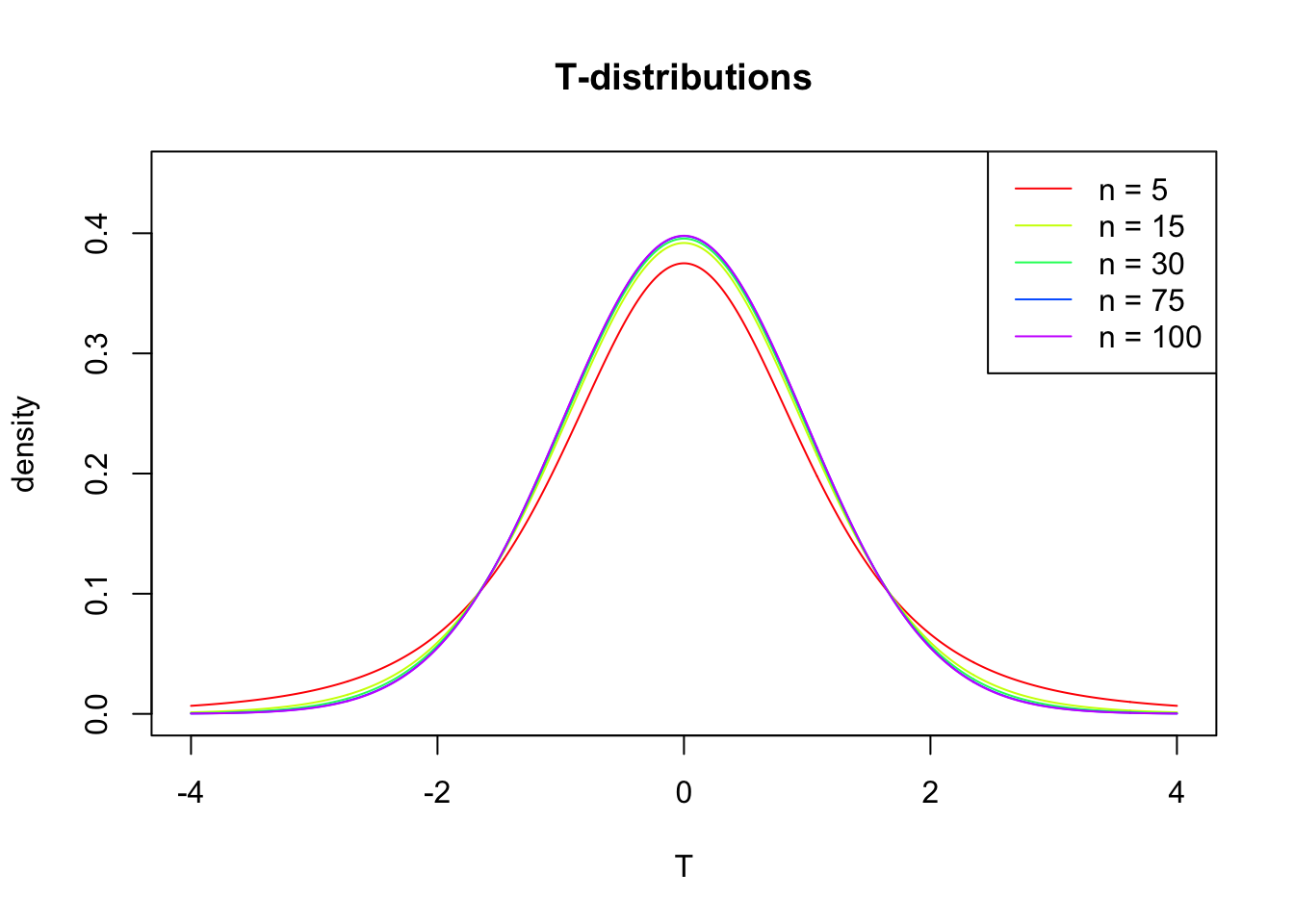
The t-distibution therefore is different for different sample sizes and converges to a standard normal distribution if sample size is large enough.
The t-distribution is defined by the probability density function (PDF):
\[\textstyle\frac{\Gamma \left(\frac{\nu+1}{2} \right)} {\sqrt{\nu\pi}\,\Gamma \left(\frac{\nu}{2} \right)} \left(1+\frac{x^2}{\nu} \right)^{-\frac{\nu+1}{2}}\!\]
where \(\nu\) is the number of degrees of freedom and \(\Gamma\) is the gamma function (Wikipedia, 2024).
Formula not exam material
End
Contact
References
- Distribution illustration generated with DALL-E by OpenAI
