Probability Models

Klinkenberg

University of Amsterdam

2024-09-09

Why do we need them

Exact approach

Coin values

Lets start simple and throw only 2 times with a fair coin. Assigning 1 for heads and 0 for tails.

The coin can only have the values 0, 1, heads or tails.

Permutation

If we throw 2 times we have the following possible outcomes.

  Toss1 Toss2
1     0     0
2     1     0
3     0     1
4     1     1

Number of heads

With frequency of heads being

  Toss1 Toss2 frequency
1     0     0         0
2     1     0         1
3     0     1         1
4     1     1         2

Probabilities

For each coin toss, disregarding the outcom, there is a .5 probability of landing heads.

  Toss1 Toss2
1   0.5   0.5
2   0.5   0.5
3   0.5   0.5
4   0.5   0.5

So for each we can specify the total probability by applying the product rule (e.g. multiplying the probabilities)

  Toss1 Toss2 probability
1   0.5   0.5        0.25
2   0.5   0.5        0.25
3   0.5   0.5        0.25
4   0.5   0.5        0.25

Which is the same for all outcomes.

Discrete probabilities

Though some outcomes occurs more often. Throwing 0 times heads, only occurs once and hence has a probability of .25. But throwing 1 times heads, can occur in two situations. So, for this situation we can add up the probabilities.

  Toss1 Toss2 frequency probability
1     0     0         0        0.25
2     1     0         1        0.25
3     0     1         1        0.25
4     1     1         2        0.25

Frequecy and probability distribution

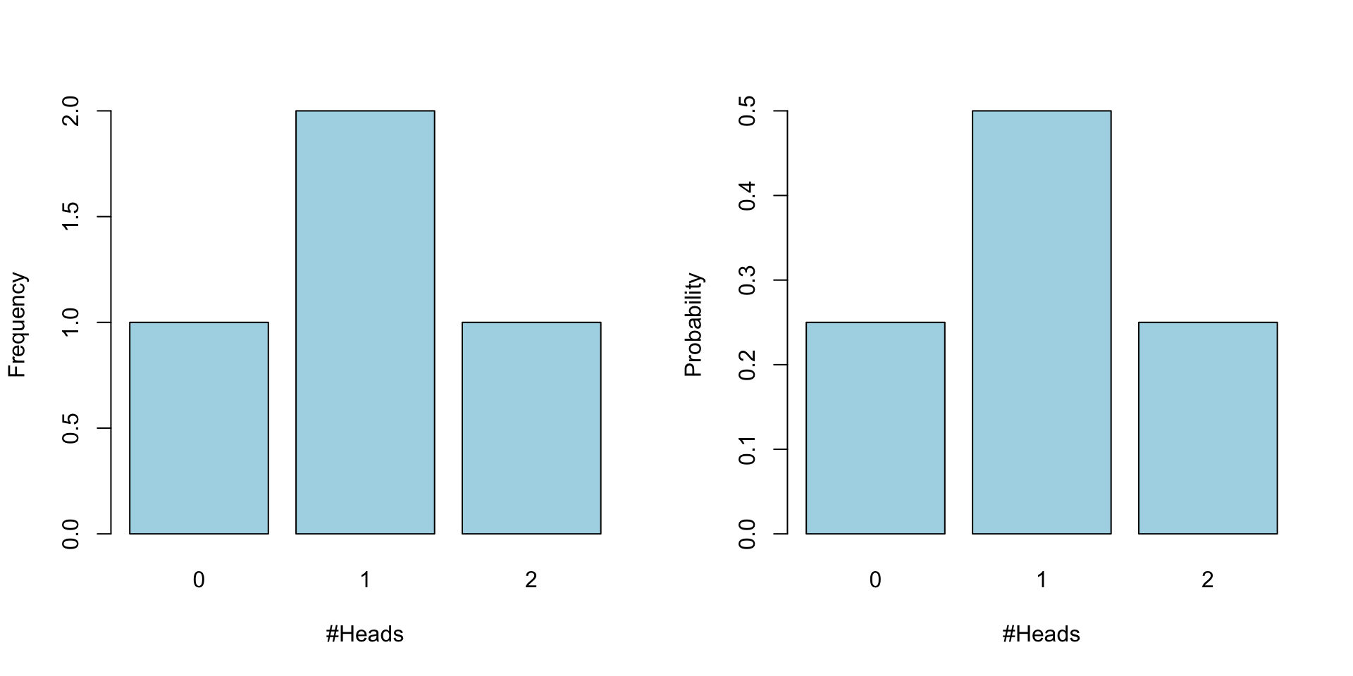
10 tosses

• Permutation
• Frequency
• Probabilities
• Probability
• Frequency and probabilities
• Cumulative probabilities

Toss1	Toss2	Toss3	Toss4	Toss5	Toss6	Toss7	Toss8	Toss9	Toss10
0.5	0.5	0.5	0.5	0.5	0.5	0.5	0.5	0.5	0.5
0.5	0.5	0.5	0.5	0.5	0.5	0.5	0.5	0.5	0.5
0.5	0.5	0.5	0.5	0.5	0.5	0.5	0.5	0.5	0.5
0.5	0.5	0.5	0.5	0.5	0.5	0.5	0.5	0.5	0.5
0.5	0.5	0.5	0.5	0.5	0.5	0.5	0.5	0.5	0.5
0.5	0.5	0.5	0.5	0.5	0.5	0.5	0.5	0.5	0.5
0.5	0.5	0.5	0.5	0.5	0.5	0.5	0.5	0.5	0.5

Toss1	Toss2	Toss3	Toss4	Toss5	Toss6	Toss7	Toss8	Toss9	Toss10	probability
0.5	0.5	0.5	0.5	0.5	0.5	0.5	0.5	0.5	0.5	0.0009766
0.5	0.5	0.5	0.5	0.5	0.5	0.5	0.5	0.5	0.5	0.0009766
0.5	0.5	0.5	0.5	0.5	0.5	0.5	0.5	0.5	0.5	0.0009766
0.5	0.5	0.5	0.5	0.5	0.5	0.5	0.5	0.5	0.5	0.0009766
0.5	0.5	0.5	0.5	0.5	0.5	0.5	0.5	0.5	0.5	0.0009766

#Heads	frequencies	Probabilities
0	1	0.0009766
1	10	0.0097656
2	45	0.0439453
3	120	0.1171875
4	210	0.2050781
5	252	0.2460938
6	210	0.2050781
7	120	0.1171875
8	45	0.0439453
9	10	0.0097656
10	1	0.0009766

Binomial distribution

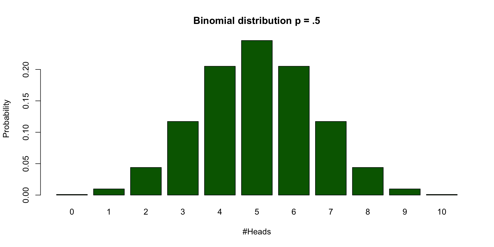
Calculate binomial probabilities

\[ {n\choose k}p^k(1-p)^{n-k}, \small {n\choose k} = \frac{n!}{k!(n-k)!} \]

• With values
• Calculations

n = 10   # Sample size
k = 0:10 # Discrete probability space
p = .5   # Probability of head

n	k	p	n!	k!	(n-k)!	(n over k)	p^k	(1-p)^(n-k)	Binom Prob
10	0	0.5	3628800	1	3628800	1	1.0000000	0.0009766	0.0009766
10	1	0.5	3628800	1	362880	10	0.5000000	0.0019531	0.0097656
10	2	0.5	3628800	2	40320	45	0.2500000	0.0039063	0.0439453
10	3	0.5	3628800	6	5040	120	0.1250000	0.0078125	0.1171875
10	4	0.5	3628800	24	720	210	0.0625000	0.0156250	0.2050781
10	5	0.5	3628800	120	120	252	0.0312500	0.0312500	0.2460938
10	6	0.5	3628800	720	24	210	0.0156250	0.0625000	0.2050781
10	7	0.5	3628800	5040	6	120	0.0078125	0.1250000	0.1171875
10	8	0.5	3628800	40320	2	45	0.0039063	0.2500000	0.0439453
10	9	0.5	3628800	362880	1	10	0.0019531	0.5000000	0.0097656
10	10	0.5	3628800	3628800	1	1	0.0009766	1.0000000	0.0009766

Warning

Formula not exam material

Bootstrapping

Sampling from your sample to approximate the sampling distribution.

My Coin tosses

my.tosses = c(1,0,0,0,0,1,0,0,0,0)

Sample from the sample

Sampling with replacement

sample(my.tosses, replace = TRUE)

 [1] 0 1 0 1 1 0 0 1 0 0

sample(my.tosses, replace = TRUE)

 [1] 0 0 0 0 0 0 0 0 0 0

sample(my.tosses, replace = TRUE)

 [1] 0 0 0 1 0 0 1 0 0 0

sample(my.tosses, replace = TRUE)

 [1] 0 0 0 0 0 0 1 0 0 0

Sampling from the sample

n.samples = 1000
n.heads = vector()

for (i in 1:n.samples) {
  my.sample <- sample(my.tosses, replace = TRUE)
  
  n.heads[i] <- sum(my.sample) 
}

5	4	3	2	1	2	5	5	3	0	1	0	2	2	2	5	2	2	1	2	1	3	3	1	1	2	0	2	2	0	2	2	2	2	3	3	0	2	2	0
1	2	1	0	3	3	1	1	5	2	3	2	0	3	6	1	3	2	2	2	1	1	1	5	1	2	1	0	3	2	3	2	2	0	1	1	2	4	1	2
1	3	3	1	4	0	6	1	2	4	3	2	5	2	4	3	1	3	2	3	3	3	5	0	0	4	0	1	0	3	4	6	3	1	0	3	4	0	1	3
0	2	3	3	0	3	2	3	5	3	3	0	1	3	2	1	1	2	1	2	4	0	1	3	1	1	3	1	0	0	0	0	2	0	4	1	1	5	1	1
1	4	1	3	4	2	3	5	2	3	2	1	2	2	1	2	0	3	0	3	2	2	1	3	1	3	1	3	2	2	2	4	1	2	3	2	1	3	0	1
2	1	1	2	2	2	4	4	2	2	1	1	3	3	1	1	1	1	2	2	0	4	0	3	1	2	1	2	5	1	2	4	1	3	1	1	2	1	1	1
4	1	1	1	1	2	1	1	1	4	3	4	1	4	1	1	4	2	2	1	1	2	1	2	1	2	1	2	3	3	5	4	4	1	2	3	3	1	4	2
1	0	4	2	4	3	3	4	0	0	2	1	2	4	2	1	1	2	1	3	3	0	2	2	2	4	2	2	0	0	4	1	2	3	2	3	0	2	3	0
2	4	3	1	4	5	2	3	2	3	1	1	3	1	4	5	1	1	3	1	3	1	1	4	5	1	0	0	3	2	1	4	4	2	2	1	2	0	2	0
3	1	5	2	1	5	3	2	0	2	2	3	4	2	3	1	2	2	1	1	1	3	0	2	1	2	3	1	2	3	1	1	2	0	1	1	3	3	1	2
5	1	2	2	2	3	1	2	0	1	2	2	1	3	1	1	2	4	2	2	1	3	1	2	3	3	2	2	1	1	3	1	0	2	3	2	1	3	2	1
2	2	2	1	1	1	1	1	2	3	1	4	2	5	3	3	3	2	2	1	2	3	1	2	2	3	1	2	5	6	1	4	2	1	1	1	3	2	2	0
1	3	3	2	1	3	1	1	3	0	1	1	3	1	0	1	4	1	2	3	1	3	3	1	2	0	2	2	1	0	4	1	1	2	2	2	2	1	1	3
3	0	4	4	3	1	2	2	2	3	3	1	1	2	1	0	1	3	4	3	3	3	3	3	2	2	2	3	5	2	3	0	3	1	4	1	1	3	3	5
2	2	3	1	1	4	3	0	2	1	1	3	3	1	2	2	3	1	3	2	3	2	0	1	4	1	1	5	2	0	3	1	3	2	3	2	2	4	2	3
4	2	1	1	3	1	1	2	1	2	2	1	2	3	3	1	2	2	4	3	3	2	3	1	1	3	3	1	2	3	0	0	2	4	2	3	2	2	1	4
2	3	3	2	5	2	1	2	0	4	3	2	3	3	2	5	0	2	2	3	0	1	4	1	3	0	2	4	6	3	3	2	1	1	4	4	3	2	3	2
1	4	4	1	1	3	2	3	2	3	2	1	0	3	2	2	2	2	3	4	3	1	0	3	0	2	4	2	3	2	3	3	1	1	1	0	3	3	0	2
2	2	2	3	1	0	1	2	2	1	3	2	1	1	2	3	1	1	2	3	0	3	2	0	2	2	1	1	2	1	2	2	3	0	1	2	3	2	0	0
3	4	3	3	3	0	2	3	1	3	1	0	1	3	2	1	0	2	1	1	2	1	2	3	2	2	4	1	4	1	1	3	2	2	1	2	2	1	1	1
1	3	2	2	2	1	3	0	4	2	1	2	1	2	4	2	4	4	1	2	4	2	2	2	1	1	2	2	3	4	2	2	2	3	0	3	0	1	1	4
2	0	2	1	0	2	1	3	3	4	0	2	0	2	3	1	2	3	2	2	2	5	0	2	2	3	0	3	3	2	2	4	2	1	3	0	2	1	4	1
1	5	3	1	1	3	5	2	2	4	2	4	3	2	3	4	3	1	2	3	2	5	0	3	3	5	2	1	0	0	2	2	4	2	3	4	1	5	0	1
2	1	2	5	4	2	2	0	3	2	0	2	0	0	4	3	3	1	4	2	2	4	1	2	4	0	2	0	1	3	1	3	3	2	2	3	2	1	0	4
1	3	4	6	1	2	2	3	1	2	3	3	0	4	0	2	0	1	1	1	2	2	3	3	4	2	3	3	1	3	0	2	0	2	2	2	2	3	0	2

Frequencies

Frequencies for number of heads per sample.

	0	1	2	3	4	5	6	7	8	9	10
Freq	106	257	294	214	90	33	6	0	0	0	0

Bootstrapped sampling distribution

Theoretical Approximations

Continuous Probability distirbutions

For all continuous probability distributions:

• Total area is always 1
• The probability of one specific test statistic is 0
• x-axis represents the test statistic
• y-axis represents the probability density

T-distribution

Gosset

William Sealy Gosset (aka Student) in 1908 (age 32)

In probability and statistics, Student’s t-distribution (or simply the t-distribution) is any member of a family of continuous probability distributions that arises when estimating the mean of a normally distributed population in situations where the sample size is small and population standard deviation is unknown.

In the English-language literature it takes its name from William Sealy Gosset’s 1908 paper in Biometrika under the pseudonym “Student”. Gosset worked at the Guinness Brewery in Dublin, Ireland, and was interested in the problems of small samples, for example the chemical properties of barley where sample sizes might be as low as 3 (Wikipedia, 2024).

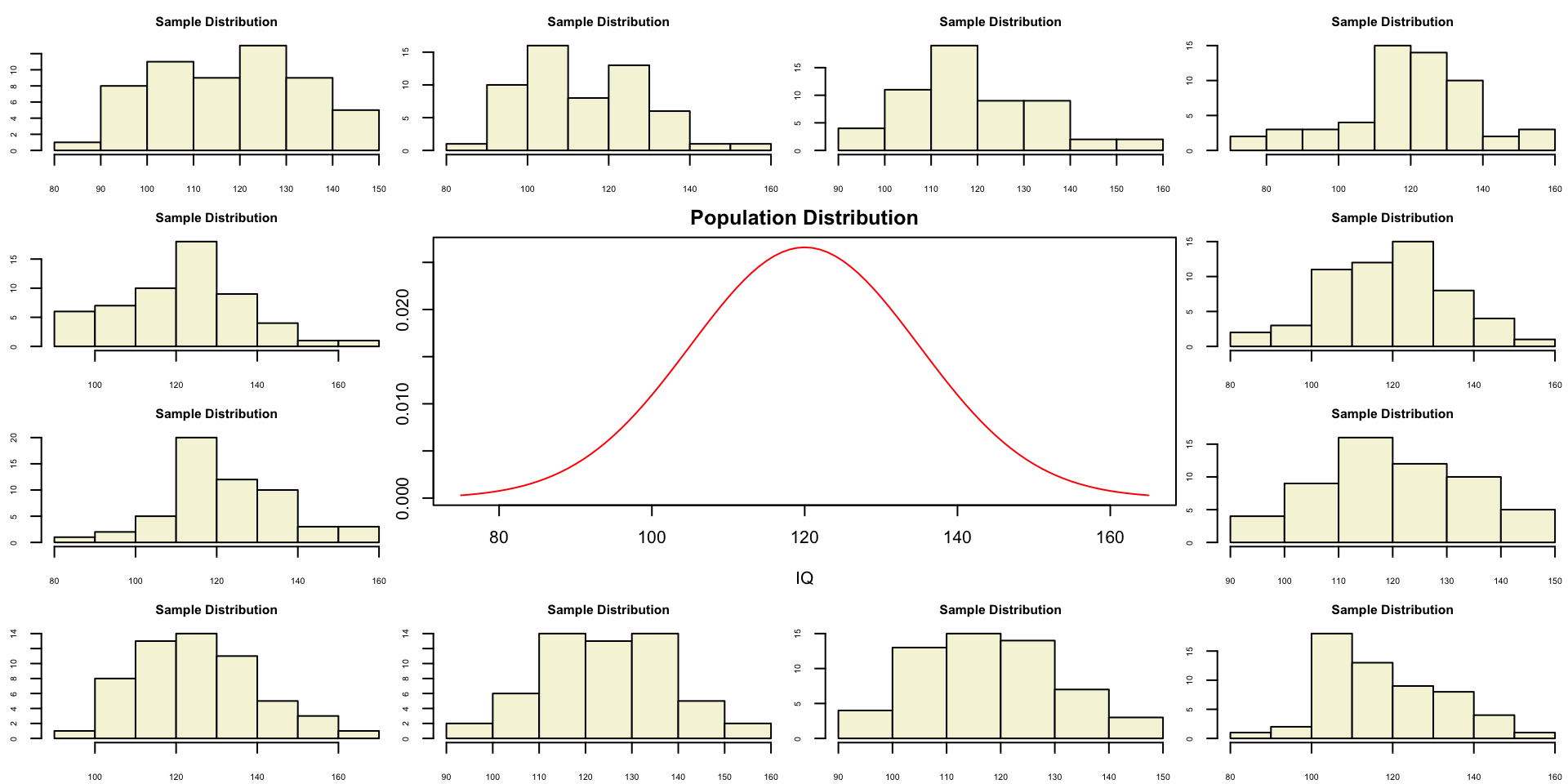
Population distribution

layout(matrix(c(2:6,1,1,7:8,1,1,9:13), 4, 4))

n  = 56    # Sample size
df = n - 1 # Degrees of freedom

mu    = 120
sigma = 15

IQ = seq(mu-45, mu+45, 1)

par(mar=c(4,2,2,0))  
plot(IQ, dnorm(IQ, mean = mu, sd = sigma), type='l', col="red", main = "Population Distribution")

n.samples = 12

for(i in 1:n.samples) {
  
  par(mar=c(2,2,2,0))  
  hist(rnorm(n, mu, sigma), main="Sample Distribution", cex.axis=.5, col="beige", cex.main = .75)
  
}

Population distribution

One sample

Let’s take a larger sample from our normal population.

x = rnorm(n, mu, sigma); x

 [1] 139.83142 120.80322 100.62919 102.66002 116.51932 115.19516 110.53936
 [8] 107.51484 102.55489  74.64233 122.80955 104.21127 136.58620 149.09940
[15] 130.07008  97.55550 145.03904 116.53760 140.85901 126.10327 118.31334
[22] 129.12780 105.23544 106.73443 127.15296 120.59382 107.67602 133.55126
[29]  96.98829 131.76937 106.14565 132.41319 110.97578 109.97020 115.70138
[36] 109.01660 123.37200 129.47526 123.61422 132.80877 108.97379 135.99577
[43] 117.41297 111.84105 112.74894 107.11346 119.83987 147.38322 123.29201
[50] 113.21733 113.69499 126.80494 109.80953 125.11899 125.11725 125.32108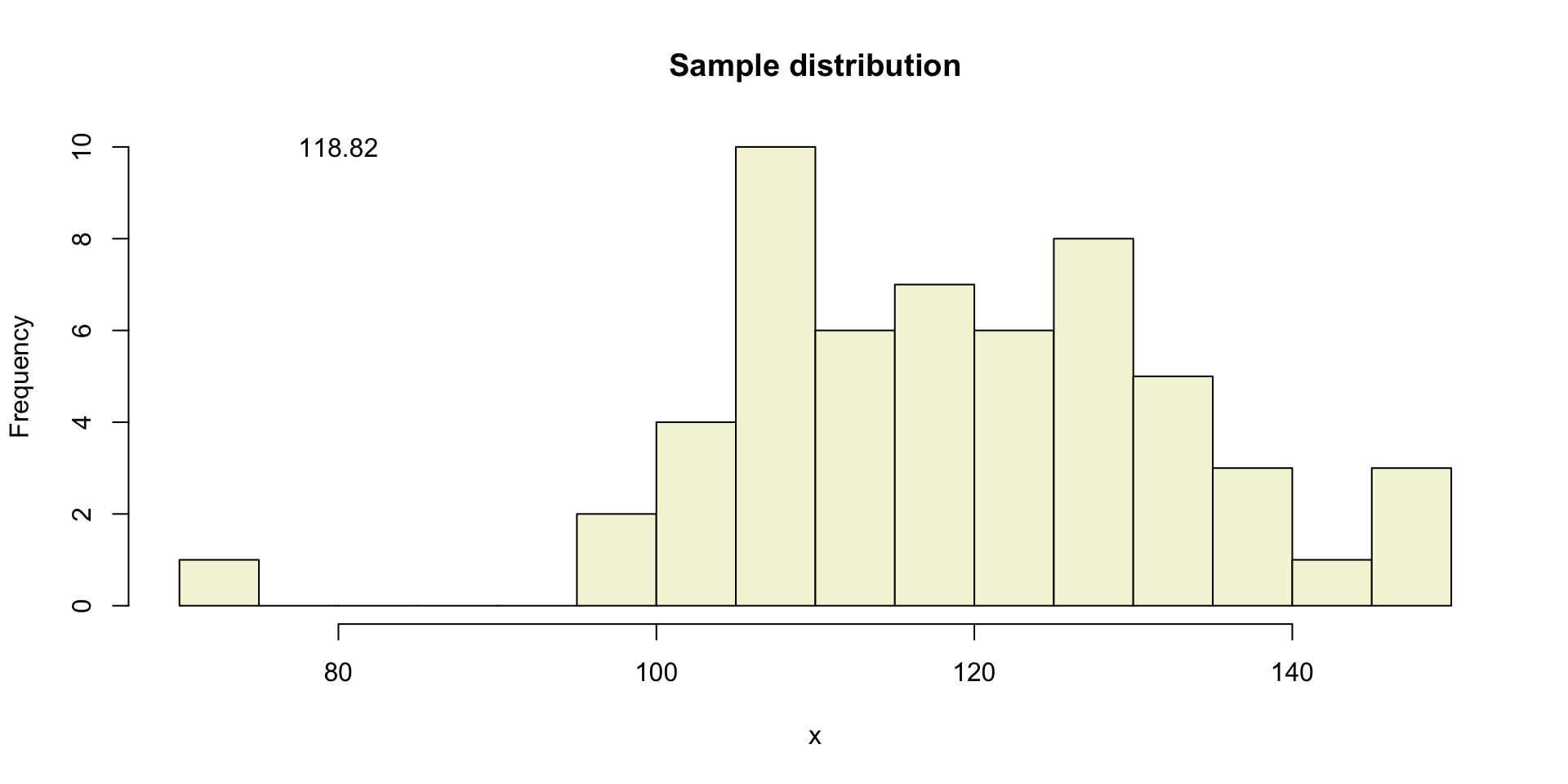

More samples

let’s take more samples.

n.samples     = 1000
mean.x.values = vector()
sd.x.values   = vector()
se.x.values   = vector()

for(i in 1:n.samples) {
  x = rnorm(n, mu, sigma)
  mean.x.values[i] = mean(x)
  se.x.values[i]   = (sd(x) / sqrt(n))
  sd.x.values[i]   = sd(x)
}

Mean and SE for all samples

mean.x.values	se.x.values
121.8412	2.218693
120.3304	1.701853
118.2349	2.006796
117.3576	2.155156
119.9086	1.940462
118.3644	1.963737

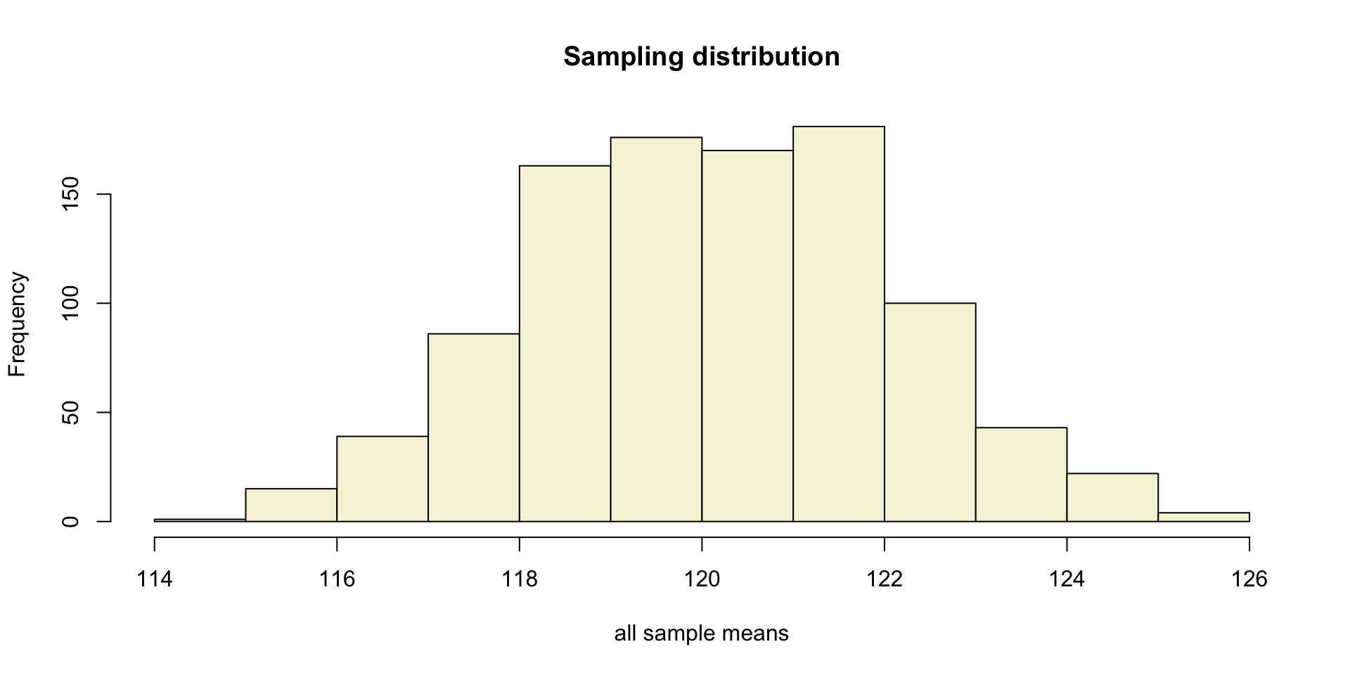
Sampling distribution

of the mean

T-statistic

\[T_{n-1} = \frac{\bar{x}-\mu}{SE_x} = \frac{\bar{x}-\mu}{s_x / \sqrt{n}}\]

So the t-statistic represents the deviation of the sample mean \(\bar{x}\) from the population mean \(\mu\), considering the sample size, expressed as the degrees of freedom \(df = n - 1\)

T-value

\[T_{n-1} = \frac{\bar{x}-\mu}{SE_x} = \frac{\bar{x}-\mu}{s_x / \sqrt{n}}\]

t = (mean(x) - mu) / (sd(x) / sqrt(n))
t

[1] -0.7974483

Calculate t-values

\[T_{n-1} = \frac{\bar{x}-\mu}{SE_x} = \frac{\bar{x}-\mu}{s_x / \sqrt{n}}\]

t.values = (mean.x.values - mu) / se.x.values

        mean.x.values  mu se.x.values   t.values
 [995,]      121.4334 120    1.926936  0.7438502
 [996,]      124.3039 120    1.805601  2.3836261
 [997,]      119.5155 120    2.095147 -0.2312486
 [998,]      119.7945 120    1.999438 -0.1028017
 [999,]      119.6265 120    1.680940 -0.2221676
[1000,]      118.1774 120    2.285533 -0.7974483

Sampling distribution t-values

The t-distribution approximates the sampling distribution, hence the name theoretical approximation.

T-distribution

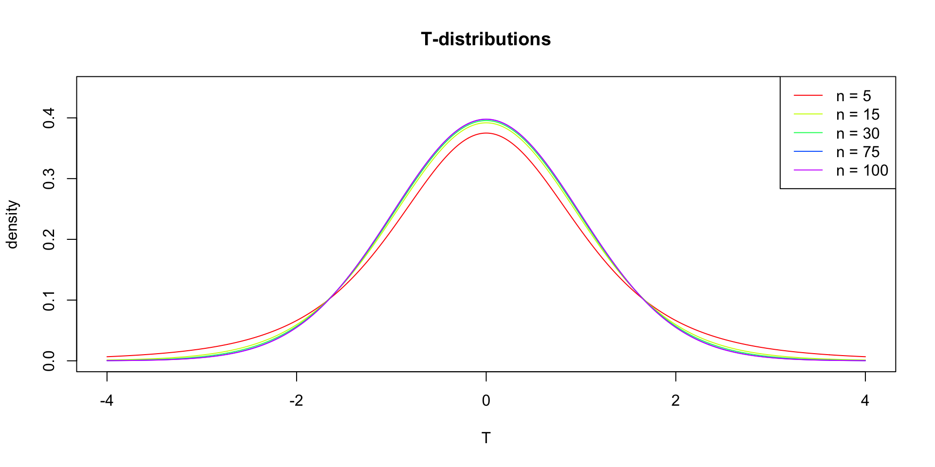
So if the population is normaly distributed (assumption of normality) the t-distribution represents the deviation of sample means from the population mean (\(\mu\)), given a certain sample size (\(df = n - 1\)).

The t-distibution therefore is different for different sample sizes and converges to a standard normal distribution if sample size is large enough.

The t-distribution is defined by the probability density function (PDF):

\[\textstyle\frac{\Gamma \left(\frac{\nu+1}{2} \right)} {\sqrt{\nu\pi}\,\Gamma \left(\frac{\nu}{2} \right)} \left(1+\frac{x^2}{\nu} \right)^{-\frac{\nu+1}{2}}\!\]

where \(\nu\) is the number of degrees of freedom and \(\Gamma\) is the gamma function (Wikipedia, 2024).

Warning

Formula not exam material

End

Contact

• Klinkenberg
• ln.AvU@grebneknilK.S
• ShKlinkenberg

CC BY-NC-SA 4.0

References

Wikipedia. (2024). Student’s t-distribution — Wikipedia, the free encyclopedia. http://en.wikipedia.org/w/index.php?title=Student's%20t-distribution&oldid=1202978121.

• Distribution illustration generated with DALL-E by OpenAI