  Toss1 Toss2
1     0     0
2     1     0
3     0     1
4 1 1Probability Models
Exact approach
Coin values
Lets start simple and throw only 2 times with a fair coin. Assigning 1 for heads and 0 for tails.
The coin can only have the values 0, 1, heads or tails.
Permutation
If we throw 2 times we have the following possible outcomes.
Number of heads
With frequency of heads being
  Toss1 Toss2 frequency
1     0     0         0
2     1     0         1
3     0     1         1
4     1     1         2
Probabilities
For each coin toss, disregarding the outcom, there is a .5 probability of landing heads.
  Toss1 Toss2
1   0.5   0.5
2   0.5   0.5
3   0.5   0.5
4   0.5   0.5
So for each we can specify the total probability by applying the product rule (e.g. multiplying the probabilities)
  Toss1 Toss2 probability
1   0.5   0.5        0.25
2   0.5   0.5        0.25
3   0.5   0.5        0.25
4   0.5   0.5        0.25
Which is the same for all outcomes.
Discrete probabilities
Though some outcomes occurs more often. Throwing 0 times heads, only occurs once and hence has a probability of .25. But throwing 1 times heads, can occur in two situations. So, for this situation we can add up the probabilities.
  Toss1 Toss2 frequency probability
1     0     0         0        0.25
2     1     0         1        0.25
3     0     1         1        0.25
4     1     1         2        0.25
Frequecy and probability distribution

10 tosses
| Toss1 | Toss2 | Toss3 | Toss4 | Toss5 | Toss6 | Toss7 | Toss8 | Toss9 | Toss10 |
|---|---|---|---|---|---|---|---|---|---|
| 0.5 | 0.5 | 0.5 | 0.5 | 0.5 | 0.5 | 0.5 | 0.5 | 0.5 | 0.5 |
| 0.5 | 0.5 | 0.5 | 0.5 | 0.5 | 0.5 | 0.5 | 0.5 | 0.5 | 0.5 |
| 0.5 | 0.5 | 0.5 | 0.5 | 0.5 | 0.5 | 0.5 | 0.5 | 0.5 | 0.5 |
| 0.5 | 0.5 | 0.5 | 0.5 | 0.5 | 0.5 | 0.5 | 0.5 | 0.5 | 0.5 |
| 0.5 | 0.5 | 0.5 | 0.5 | 0.5 | 0.5 | 0.5 | 0.5 | 0.5 | 0.5 |
| 0.5 | 0.5 | 0.5 | 0.5 | 0.5 | 0.5 | 0.5 | 0.5 | 0.5 | 0.5 |
| 0.5 | 0.5 | 0.5 | 0.5 | 0.5 | 0.5 | 0.5 | 0.5 | 0.5 | 0.5 |
| Toss1 | Toss2 | Toss3 | Toss4 | Toss5 | Toss6 | Toss7 | Toss8 | Toss9 | Toss10 | probability |
|---|---|---|---|---|---|---|---|---|---|---|
| 0.5 | 0.5 | 0.5 | 0.5 | 0.5 | 0.5 | 0.5 | 0.5 | 0.5 | 0.5 | 0.0009766 |
| 0.5 | 0.5 | 0.5 | 0.5 | 0.5 | 0.5 | 0.5 | 0.5 | 0.5 | 0.5 | 0.0009766 |
| 0.5 | 0.5 | 0.5 | 0.5 | 0.5 | 0.5 | 0.5 | 0.5 | 0.5 | 0.5 | 0.0009766 |
| 0.5 | 0.5 | 0.5 | 0.5 | 0.5 | 0.5 | 0.5 | 0.5 | 0.5 | 0.5 | 0.0009766 |
| 0.5 | 0.5 | 0.5 | 0.5 | 0.5 | 0.5 | 0.5 | 0.5 | 0.5 | 0.5 | 0.0009766 |
| #Heads | frequencies | Probabilities |
|---|---|---|
| 0 | 1 | 0.0009766 |
| 1 | 10 | 0.0097656 |
| 2 | 45 | 0.0439453 |
| 3 | 120 | 0.1171875 |
| 4 | 210 | 0.2050781 |
| 5 | 252 | 0.2460938 |
| 6 | 210 | 0.2050781 |
| 7 | 120 | 0.1171875 |
| 8 | 45 | 0.0439453 |
| 9 | 10 | 0.0097656 |
| 10 | 1 | 0.0009766 |
Binomial distribution

Calculate binomial probabilities
\[ {n\choose k}p^k(1-p)^{n-k}, \small {n\choose k} = \frac{n!}{k!(n-k)!} \]
n = 10   # Sample size
k = 0:10 # Discrete probability space
p = .5 # Probability of head| n | k | p | n! | k! | (n-k)! | (n over k) | p^k | (1-p)^(n-k) | Binom Prob |
|---|---|---|---|---|---|---|---|---|---|
| 10 | 0 | 0.5 | 3628800 | 1 | 3628800 | 1 | 1.0000000 | 0.0009766 | 0.0009766 |
| 10 | 1 | 0.5 | 3628800 | 1 | 362880 | 10 | 0.5000000 | 0.0019531 | 0.0097656 |
| 10 | 2 | 0.5 | 3628800 | 2 | 40320 | 45 | 0.2500000 | 0.0039063 | 0.0439453 |
| 10 | 3 | 0.5 | 3628800 | 6 | 5040 | 120 | 0.1250000 | 0.0078125 | 0.1171875 |
| 10 | 4 | 0.5 | 3628800 | 24 | 720 | 210 | 0.0625000 | 0.0156250 | 0.2050781 |
| 10 | 5 | 0.5 | 3628800 | 120 | 120 | 252 | 0.0312500 | 0.0312500 | 0.2460938 |
| 10 | 6 | 0.5 | 3628800 | 720 | 24 | 210 | 0.0156250 | 0.0625000 | 0.2050781 |
| 10 | 7 | 0.5 | 3628800 | 5040 | 6 | 120 | 0.0078125 | 0.1250000 | 0.1171875 |
| 10 | 8 | 0.5 | 3628800 | 40320 | 2 | 45 | 0.0039063 | 0.2500000 | 0.0439453 |
| 10 | 9 | 0.5 | 3628800 | 362880 | 1 | 10 | 0.0019531 | 0.5000000 | 0.0097656 |
| 10 | 10 | 0.5 | 3628800 | 3628800 | 1 | 1 | 0.0009766 | 1.0000000 | 0.0009766 |
Bootstrapping
Sampling from your sample to approximate the sampling distribution.
My Coin tosses
my.tosses = c(0,1,0,1,0,0,0,0,0,0)Sample from the sample
Sampling with replacement
sample(my.tosses, replace = TRUE) [1] 0 1 0 0 0 0 1 0 0 0sample(my.tosses, replace = TRUE) [1] 0 1 0 0 0 0 0 0 0 0sample(my.tosses, replace = TRUE) [1] 0 0 0 1 1 0 0 0 1 0sample(my.tosses, replace = TRUE) [1] 0 0 1 1 1 1 0 0 0 0Sampling from the sample
n.samples = 1000
n.heads = vector()

for (i in 1:n.samples) {
  my.sample <- sample(my.tosses, replace = TRUE)

  n.heads[i] <- sum(my.sample)
}| 1 | 2 | 1 | 1 | 2 | 2 | 3 | 0 | 2 | 1 | 3 | 6 | 4 | 1 | 5 | 1 | 0 | 2 | 2 | 3 | 2 | 4 | 1 | 1 | 2 | 2 | 2 | 1 | 3 | 2 | 3 | 1 | 1 | 3 | 1 | 3 | 3 | 2 | 2 | 2 |
| 2 | 3 | 2 | 3 | 2 | 2 | 2 | 2 | 2 | 0 | 1 | 0 | 3 | 5 | 2 | 2 | 4 | 3 | 1 | 1 | 3 | 4 | 4 | 5 | 3 | 1 | 0 | 1 | 2 | 1 | 4 | 5 | 2 | 2 | 1 | 0 | 1 | 1 | 3 | 3 |
| 0 | 1 | 3 | 3 | 2 | 1 | 2 | 2 | 1 | 3 | 1 | 1 | 2 | 3 | 1 | 1 | 2 | 2 | 0 | 2 | 3 | 2 | 4 | 2 | 3 | 0 | 3 | 4 | 2 | 2 | 2 | 4 | 2 | 1 | 0 | 2 | 1 | 3 | 0 | 1 |
| 3 | 2 | 2 | 1 | 0 | 1 | 2 | 6 | 4 | 2 | 3 | 2 | 3 | 3 | 3 | 1 | 4 | 0 | 2 | 2 | 3 | 3 | 3 | 3 | 2 | 2 | 1 | 1 | 2 | 4 | 3 | 1 | 0 | 0 | 5 | 4 | 5 | 0 | 2 | 1 |
| 3 | 2 | 0 | 3 | 3 | 4 | 1 | 2 | 4 | 3 | 3 | 0 | 0 | 3 | 4 | 2 | 2 | 1 | 2 | 3 | 2 | 0 | 1 | 1 | 2 | 1 | 1 | 0 | 3 | 3 | 1 | 3 | 3 | 2 | 2 | 6 | 1 | 3 | 1 | 1 |
| 2 | 2 | 1 | 2 | 1 | 1 | 1 | 0 | 1 | 2 | 1 | 5 | 2 | 3 | 0 | 2 | 2 | 2 | 1 | 3 | 0 | 3 | 3 | 4 | 5 | 1 | 3 | 2 | 1 | 6 | 2 | 0 | 2 | 4 | 6 | 2 | 2 | 3 | 4 | 2 |
| 4 | 3 | 0 | 4 | 1 | 1 | 1 | 2 | 1 | 2 | 2 | 1 | 4 | 5 | 2 | 1 | 3 | 1 | 1 | 1 | 5 | 0 | 2 | 1 | 3 | 3 | 2 | 1 | 3 | 1 | 5 | 0 | 4 | 2 | 2 | 3 | 2 | 2 | 1 | 4 |
| 0 | 0 | 3 | 2 | 3 | 0 | 3 | 1 | 3 | 2 | 3 | 2 | 4 | 3 | 0 | 3 | 3 | 0 | 1 | 0 | 4 | 1 | 3 | 1 | 2 | 2 | 3 | 2 | 3 | 1 | 2 | 2 | 1 | 3 | 5 | 3 | 2 | 0 | 0 | 0 |
| 1 | 3 | 2 | 2 | 2 | 1 | 5 | 1 | 2 | 1 | 6 | 1 | 0 | 2 | 2 | 4 | 2 | 2 | 2 | 3 | 2 | 2 | 4 | 3 | 1 | 1 | 5 | 2 | 1 | 4 | 3 | 3 | 1 | 0 | 2 | 1 | 3 | 2 | 2 | 4 |
| 2 | 3 | 2 | 0 | 1 | 2 | 2 | 3 | 0 | 2 | 3 | 1 | 2 | 1 | 1 | 1 | 2 | 2 | 3 | 4 | 1 | 4 | 0 | 0 | 1 | 2 | 2 | 2 | 1 | 2 | 4 | 5 | 1 | 2 | 3 | 3 | 1 | 1 | 5 | 2 |
| 4 | 2 | 3 | 3 | 1 | 3 | 2 | 2 | 1 | 2 | 3 | 0 | 5 | 3 | 2 | 2 | 2 | 0 | 1 | 3 | 1 | 2 | 2 | 2 | 1 | 2 | 2 | 0 | 1 | 3 | 3 | 3 | 3 | 2 | 1 | 5 | 1 | 3 | 2 | 2 |
| 1 | 0 | 1 | 0 | 3 | 1 | 2 | 2 | 2 | 4 | 2 | 2 | 0 | 3 | 3 | 1 | 4 | 3 | 0 | 3 | 1 | 1 | 0 | 2 | 2 | 1 | 0 | 1 | 3 | 3 | 1 | 2 | 1 | 2 | 1 | 2 | 1 | 1 | 3 | 2 |
| 2 | 3 | 3 | 2 | 2 | 0 | 2 | 2 | 2 | 2 | 1 | 2 | 2 | 3 | 2 | 1 | 2 | 2 | 2 | 2 | 2 | 1 | 3 | 1 | 3 | 2 | 2 | 2 | 1 | 3 | 3 | 1 | 2 | 3 | 1 | 2 | 1 | 2 | 2 | 2 |
| 1 | 1 | 2 | 1 | 2 | 0 | 2 | 3 | 0 | 2 | 1 | 3 | 0 | 3 | 4 | 4 | 3 | 2 | 2 | 3 | 1 | 2 | 4 | 1 | 5 | 2 | 3 | 3 | 0 | 2 | 1 | 1 | 2 | 1 | 1 | 0 | 2 | 3 | 3 | 6 |
| 2 | 2 | 1 | 1 | 1 | 0 | 2 | 5 | 3 | 1 | 3 | 2 | 4 | 5 | 0 | 1 | 2 | 2 | 0 | 3 | 2 | 2 | 0 | 3 | 2 | 2 | 2 | 1 | 2 | 2 | 2 | 1 | 1 | 3 | 1 | 4 | 2 | 0 | 3 | 3 |
| 1 | 3 | 3 | 1 | 1 | 1 | 2 | 3 | 2 | 0 | 1 | 1 | 2 | 1 | 1 | 2 | 3 | 0 | 1 | 2 | 4 | 4 | 0 | 2 | 1 | 1 | 2 | 2 | 2 | 6 | 1 | 3 | 1 | 5 | 3 | 4 | 3 | 4 | 2 | 0 |
| 5 | 3 | 2 | 4 | 3 | 4 | 5 | 2 | 2 | 4 | 1 | 2 | 1 | 1 | 2 | 1 | 1 | 1 | 2 | 0 | 3 | 3 | 1 | 2 | 3 | 4 | 1 | 3 | 4 | 2 | 1 | 2 | 2 | 2 | 4 | 1 | 2 | 3 | 3 | 2 |
| 2 | 0 | 1 | 2 | 2 | 0 | 3 | 2 | 3 | 1 | 2 | 0 | 1 | 1 | 2 | 3 | 3 | 1 | 3 | 1 | 1 | 2 | 0 | 5 | 4 | 1 | 2 | 3 | 1 | 1 | 1 | 2 | 2 | 4 | 4 | 1 | 1 | 2 | 0 | 1 |
| 2 | 3 | 0 | 4 | 4 | 1 | 3 | 2 | 3 | 4 | 2 | 1 | 2 | 3 | 0 | 3 | 2 | 4 | 1 | 4 | 2 | 2 | 1 | 1 | 3 | 2 | 5 | 3 | 4 | 2 | 1 | 2 | 5 | 2 | 4 | 4 | 1 | 4 | 3 | 3 |
| 1 | 3 | 3 | 1 | 2 | 0 | 1 | 2 | 2 | 2 | 4 | 6 | 2 | 2 | 1 | 0 | 3 | 3 | 5 | 3 | 2 | 6 | 4 | 1 | 3 | 1 | 2 | 1 | 1 | 1 | 4 | 2 | 2 | 1 | 0 | 3 | 2 | 3 | 1 | 1 |
| 2 | 2 | 0 | 2 | 4 | 1 | 2 | 1 | 2 | 2 | 3 | 3 | 1 | 2 | 3 | 4 | 1 | 1 | 3 | 2 | 3 | 1 | 2 | 2 | 2 | 2 | 1 | 0 | 1 | 3 | 2 | 1 | 3 | 2 | 1 | 0 | 3 | 1 | 1 | 2 |
| 2 | 2 | 5 | 1 | 0 | 3 | 0 | 3 | 2 | 3 | 1 | 4 | 1 | 1 | 4 | 1 | 1 | 4 | 1 | 1 | 2 | 3 | 0 | 2 | 2 | 0 | 0 | 3 | 2 | 0 | 1 | 2 | 1 | 2 | 2 | 1 | 0 | 2 | 1 | 5 |
| 1 | 1 | 3 | 2 | 2 | 2 | 2 | 4 | 1 | 1 | 0 | 0 | 1 | 2 | 5 | 3 | 2 | 2 | 1 | 1 | 1 | 3 | 0 | 1 | 2 | 2 | 3 | 4 | 3 | 3 | 1 | 4 | 3 | 3 | 1 | 5 | 1 | 3 | 0 | 1 |
| 1 | 1 | 1 | 2 | 3 | 1 | 4 | 2 | 1 | 3 | 1 | 3 | 2 | 2 | 2 | 4 | 5 | 3 | 3 | 2 | 1 | 2 | 1 | 3 | 1 | 2 | 2 | 4 | 1 | 4 | 2 | 1 | 4 | 4 | 3 | 2 | 1 | 2 | 5 | 2 |
| 1 | 3 | 2 | 3 | 2 | 3 | 4 | 2 | 1 | 3 | 1 | 1 | 2 | 2 | 3 | 4 | 0 | 2 | 1 | 3 | 1 | 1 | 2 | 3 | 1 | 1 | 2 | 4 | 1 | 2 | 2 | 1 | 3 | 1 | 5 | 2 | 2 | 1 | 2 | 2 |
Frequencies
Frequencies for number of heads per sample.
| 0 | 1 | 2 | 3 | 4 | 5 | 6 | 7 | 8 | 9 | 10 | |
|---|---|---|---|---|---|---|---|---|---|---|---|
| Freq | 93 | 263 | 315 | 201 | 83 | 35 | 10 | 0 | 0 | 0 | 0 |
Bootstrapped sampling distribution

Theoretical Approximations
Continuous Probability distirbutions

For all continuous probability distributions:
- Total area is always 1
- The probability of one specific test statistic is 0
- x-axis represents the test statistic
- y-axis represents the probability density
T-distribution
Gosset

In probability and statistics, Student’s t-distribution (or simply the t-distribution) is any member of a family of continuous probability distributions that arises when estimating the mean of a normally distributed population in situations where the sample size is small and population standard deviation is unknown.
In the English-language literature it takes its name from William Sealy Gosset’s 1908 paper in Biometrika under the pseudonym “Student”. Gosset worked at the Guinness Brewery in Dublin, Ireland, and was interested in the problems of small samples, for example the chemical properties of barley where sample sizes might be as low as 3 (Wikipedia, 2024).
Population distribution
layout(matrix(c(2:6,1,1,7:8,1,1,9:13), 4, 4))

n  = 56    # Sample size
df = n - 1 # Degrees of freedom

mu    = 120
sigma = 15

IQ = seq(mu-45, mu+45, 1)

par(mar=c(4,2,2,0))
plot(IQ, dnorm(IQ, mean = mu, sd = sigma), type='l', col="red", main = "Population Distribution")

n.samples = 12

for(i in 1:n.samples) {

  par(mar=c(2,2,2,0))
  hist(rnorm(n, mu, sigma), main="Sample Distribution", cex.axis=.5, col="beige", cex.main = .75)

}
One sample
Let’s take a larger sample from our normal population.
x = rnorm(n, mu, sigma); x [1] 107.17927 130.80676 127.94839 141.33349 122.89934 77.66882 116.82787
[8] 133.02924 109.97133 133.56940 122.49528 118.55665 116.11118 110.04206
[15] 113.68917 133.01632 131.32582 121.12561 110.81535 112.13214 112.34638
[22] 124.44749 161.89195 127.07004 102.62866 96.62265 131.26846 117.60728
[29] 136.09720 135.64733 106.29816 116.99422 109.27281 110.40999 109.66679
[36] 123.89073 144.38404 109.68744 118.86466 113.77315 116.06298 133.47985
[43] 95.53884 124.39871 118.32193 123.64072 113.10669 84.83373 129.23723
[50] 86.26019 121.81305 138.04168 119.12822 113.19637 117.03577 141.52632
More samples
let’s take more samples.
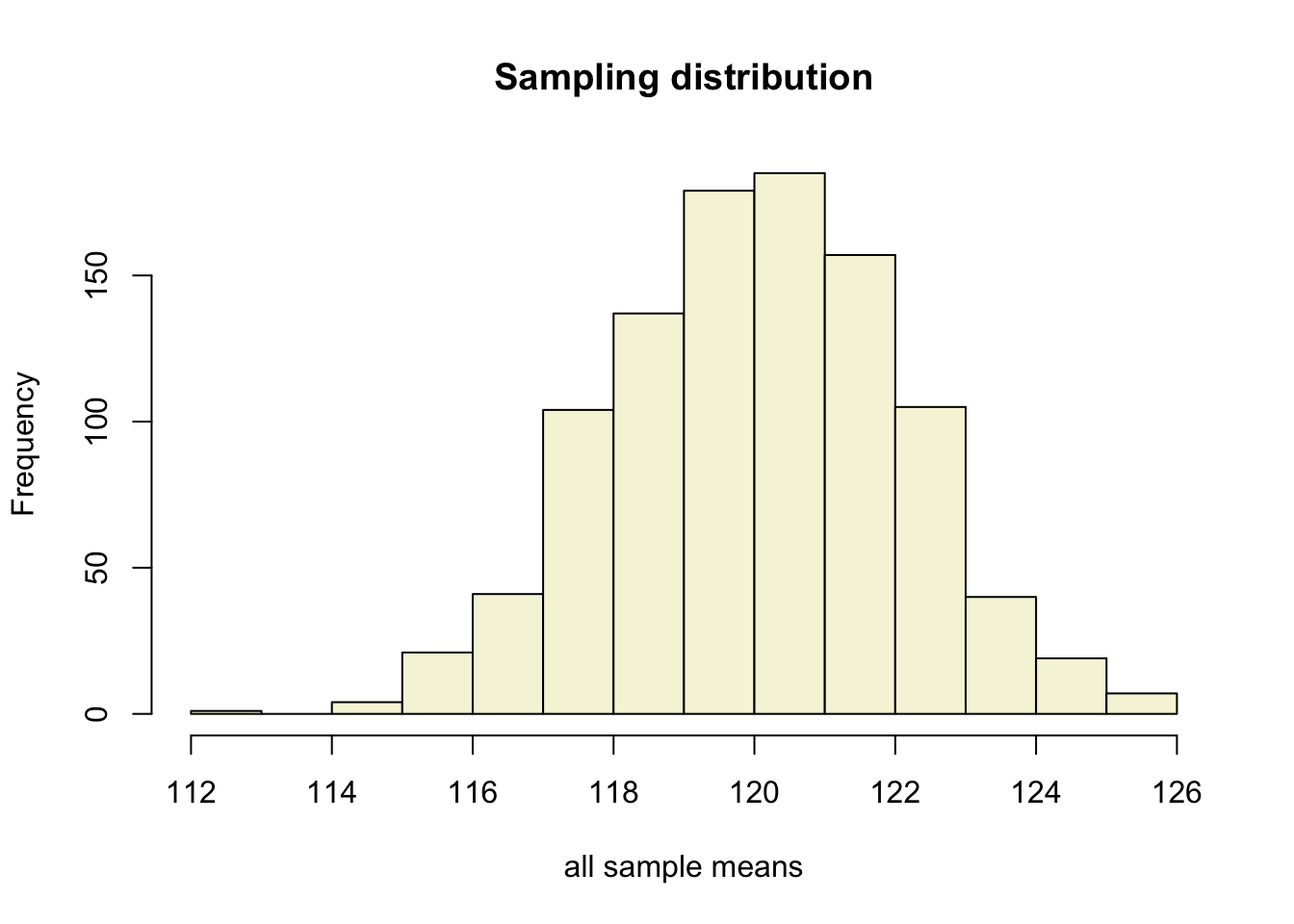
Mean and SE for all samples
| mean.x.values | se.x.values |
|---|---|
| 122.0378 | 2.178401 |
| 118.2087 | 2.046157 |
| 117.3111 | 1.852351 |
| 117.3727 | 1.862840 |
| 116.0319 | 1.867772 |
| 119.0341 | 2.270794 |
Sampling distribution
of the mean
T-statistic
\[T_{n-1} = \frac{\bar{x}-\mu}{SE_x} = \frac{\bar{x}-\mu}{s_x / \sqrt{n}}\]
So the t-statistic represents the deviation of the sample mean \(\bar{x}\) from the population mean \(\mu\), considering the sample size, expressed as the degrees of freedom \(df = n - 1\)
T-value
\[T_{n-1} = \frac{\bar{x}-\mu}{SE_x} = \frac{\bar{x}-\mu}{s_x / \sqrt{n}}\]
t = (mean(x) - mu) / (sd(x) / sqrt(n))
t
[1] 0.2487238Calculate t-values
\[T_{n-1} = \frac{\bar{x}-\mu}{SE_x} = \frac{\bar{x}-\mu}{s_x / \sqrt{n}}\]
t.values = (mean.x.values - mu) / se.x.values mean.x.values mu se.x.values t.values
[995,] 115.9547 120 2.399117 -1.68616959
[996,] 119.8866 120 2.061135 -0.05503363
[997,] 118.7975 120 2.141113 -0.56164382
[998,] 120.4509 120 1.986195 0.22703385
[999,] 118.1819 120 2.337895 -0.77765053
[1000,] 120.4615 120 1.855412 0.24872380Sampling distribution t-values

T-distribution
So if the population is normaly distributed (assumption of normality) the t-distribution represents the deviation of sample means from the population mean (\(\mu\)), given a certain sample size (\(df = n - 1\)).
The t-distibution therefore is different for different sample sizes and converges to a standard normal distribution if sample size is large enough.
The t-distribution is defined by the probability density function (PDF):
\[\textstyle\frac{\Gamma \left(\frac{\nu+1}{2} \right)} {\sqrt{\nu\pi}\,\Gamma \left(\frac{\nu}{2} \right)} \left(1+\frac{x^2}{\nu} \right)^{-\frac{\nu+1}{2}}\!\]
where \(\nu\) is the number of degrees of freedom and \(\Gamma\) is the gamma function (Wikipedia, 2024).
Warning
Formula not exam material

One or two sided
Two sided
- \(H_A: \bar{x} \neq \mu\)
One sided
- \(H_A: \bar{x} > \mu\)
- \(H_A: \bar{x} < \mu\)

End
Contact

References
Wikipedia. (2024). Student’s t-distribution — Wikipedia, the free encyclopedia. http://en.wikipedia.org/w/index.php?title=Student's%20t-distribution&oldid=1202978121.