  Toss1 Toss2
1     0     0
2     1     0
3     0     1
4 1 1Probability Models
2024-02-12
Frequecy and probability distribution

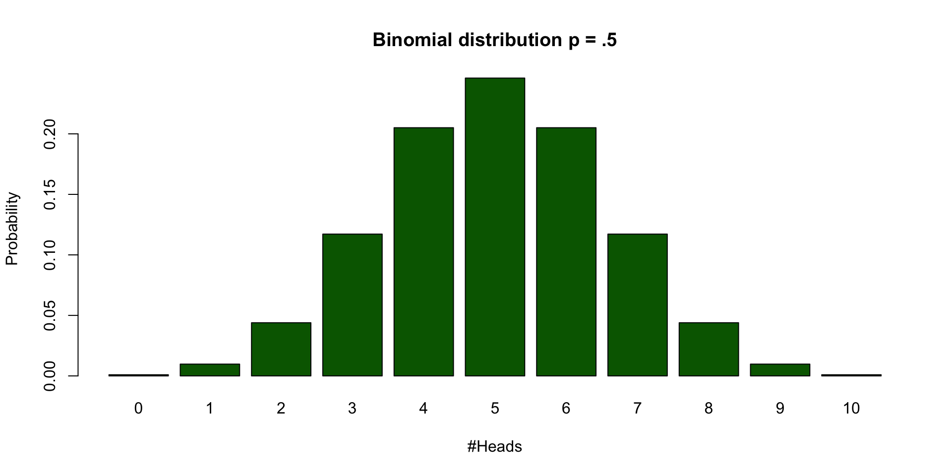
Binomial distribution
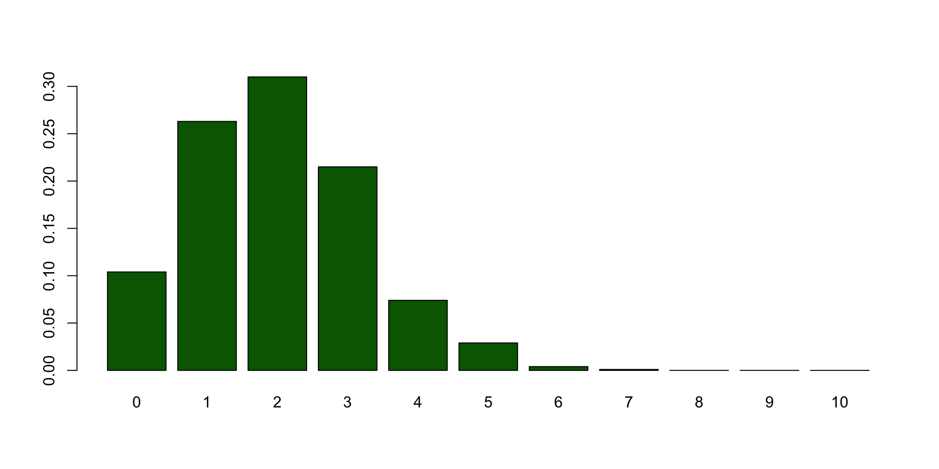
Bootstrapped sampling distribution
Continuous Probability distirbutions
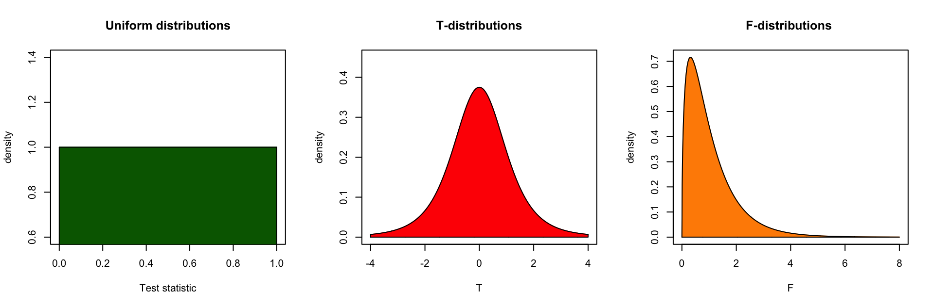
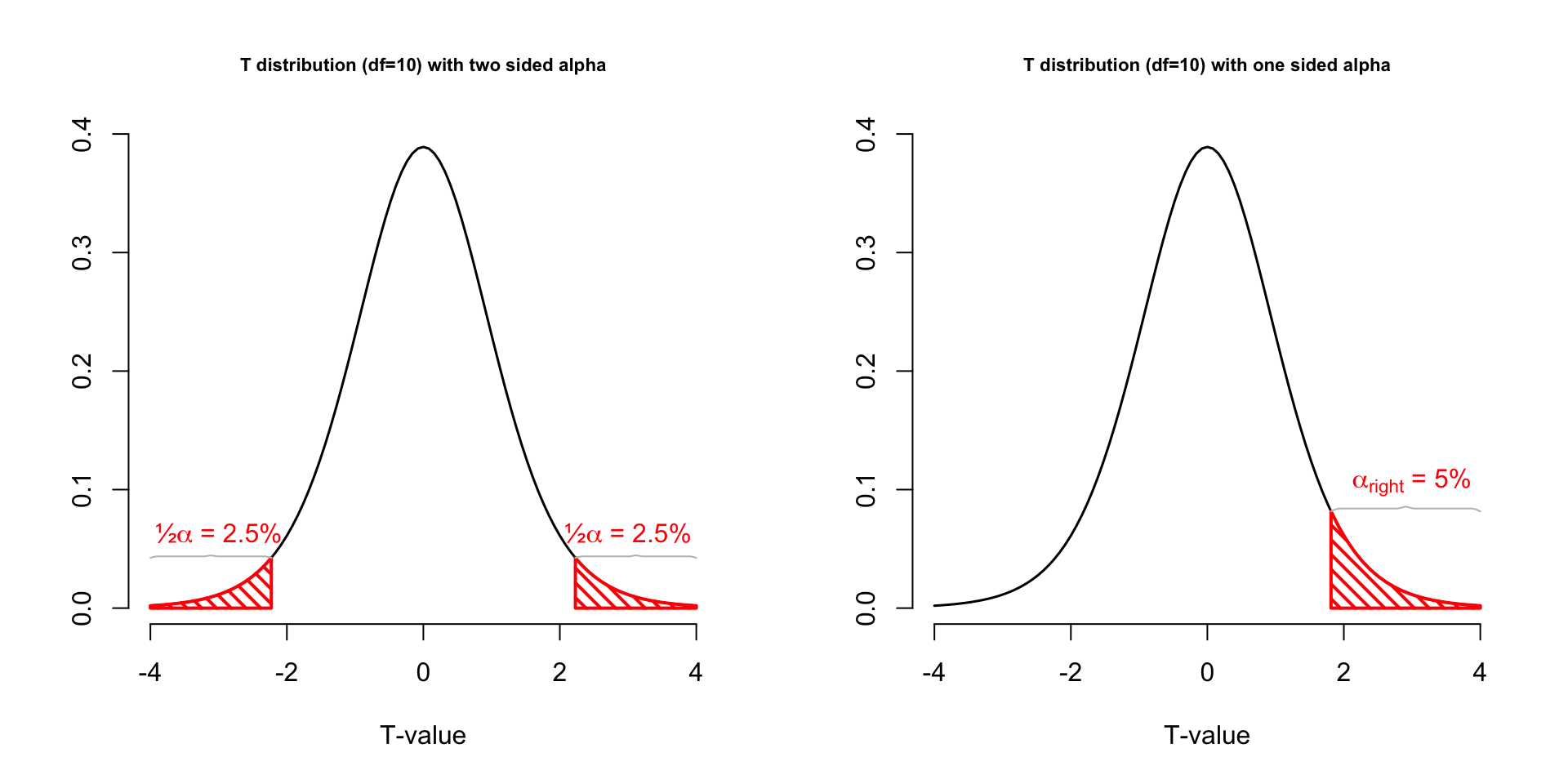
For all continuous probability distributions:
- Total area is always 1
- The probability of one specific test statistic is 0
- x-axis represents the test statistic
- y-axis represents the probability density
Gosset

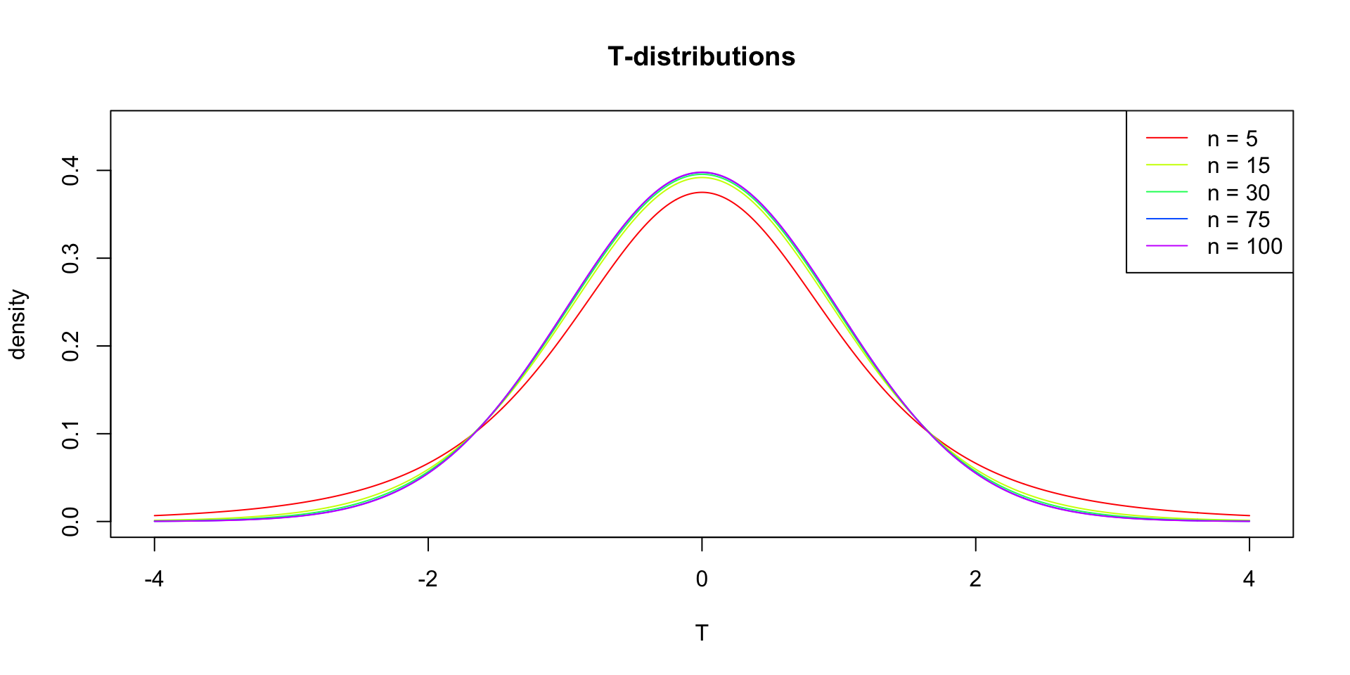
In probability and statistics, Student’s t-distribution (or simply the t-distribution) is any member of a family of continuous probability distributions that arises when estimating the mean of a normally distributed population in situations where the sample size is small and population standard deviation is unknown.
In the English-language literature it takes its name from William Sealy Gosset’s 1908 paper in Biometrika under the pseudonym “Student”. Gosset worked at the Guinness Brewery in Dublin, Ireland, and was interested in the problems of small samples, for example the chemical properties of barley where sample sizes might be as low as 3 (Wikipedia, 2024).
Population distribution
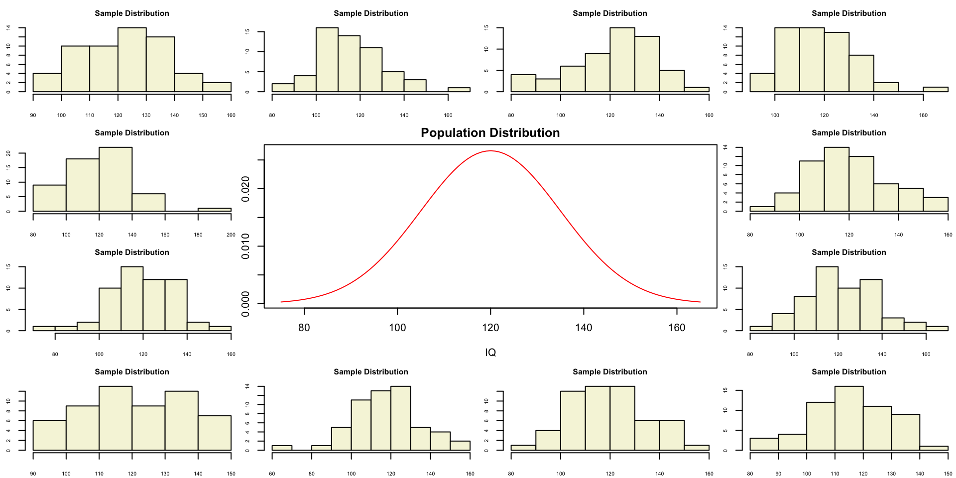
One sample
Let’s take a larger sample from our normal population.
 [1] 107.23685 127.41511 114.49546 117.95965 114.28153 103.07176 111.25836
 [8] 113.32382 119.02879 106.59907 126.02548 148.09688 100.41463 115.35363
[15] 110.83483 119.10494 145.80933 112.99751 124.73989  96.95211 133.51865
[22] 115.11211 112.44197 133.23333 127.44063 117.51603 110.32868  97.04325
[29] 107.35497 144.51702 112.78471 111.58268 128.19846 103.32059 116.82780
[36] 105.43609 117.68510  99.12848 113.08409 120.31098  84.90971 128.78364
[43] 141.29826 113.82271  88.68238 132.32723 116.03553 124.13257 107.46536
[50] 122.29764 131.74950 115.54641  92.64111  95.68900 107.86958 102.73153
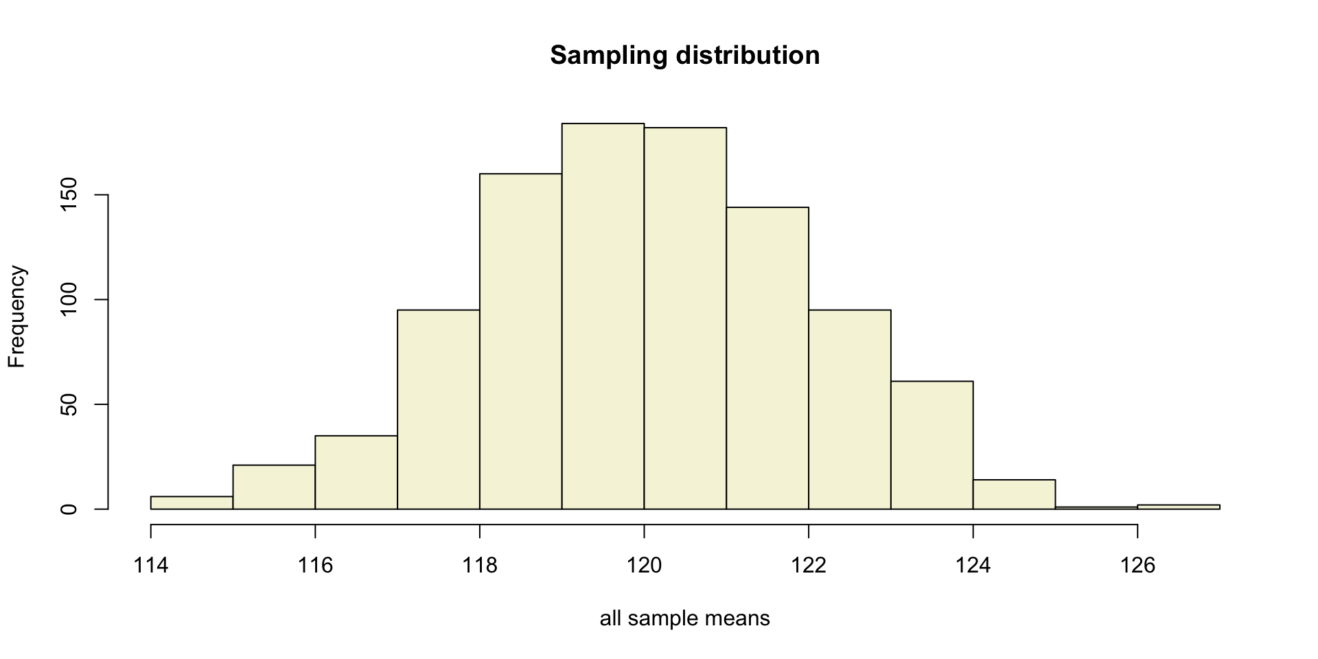
Sampling distribution
of the mean
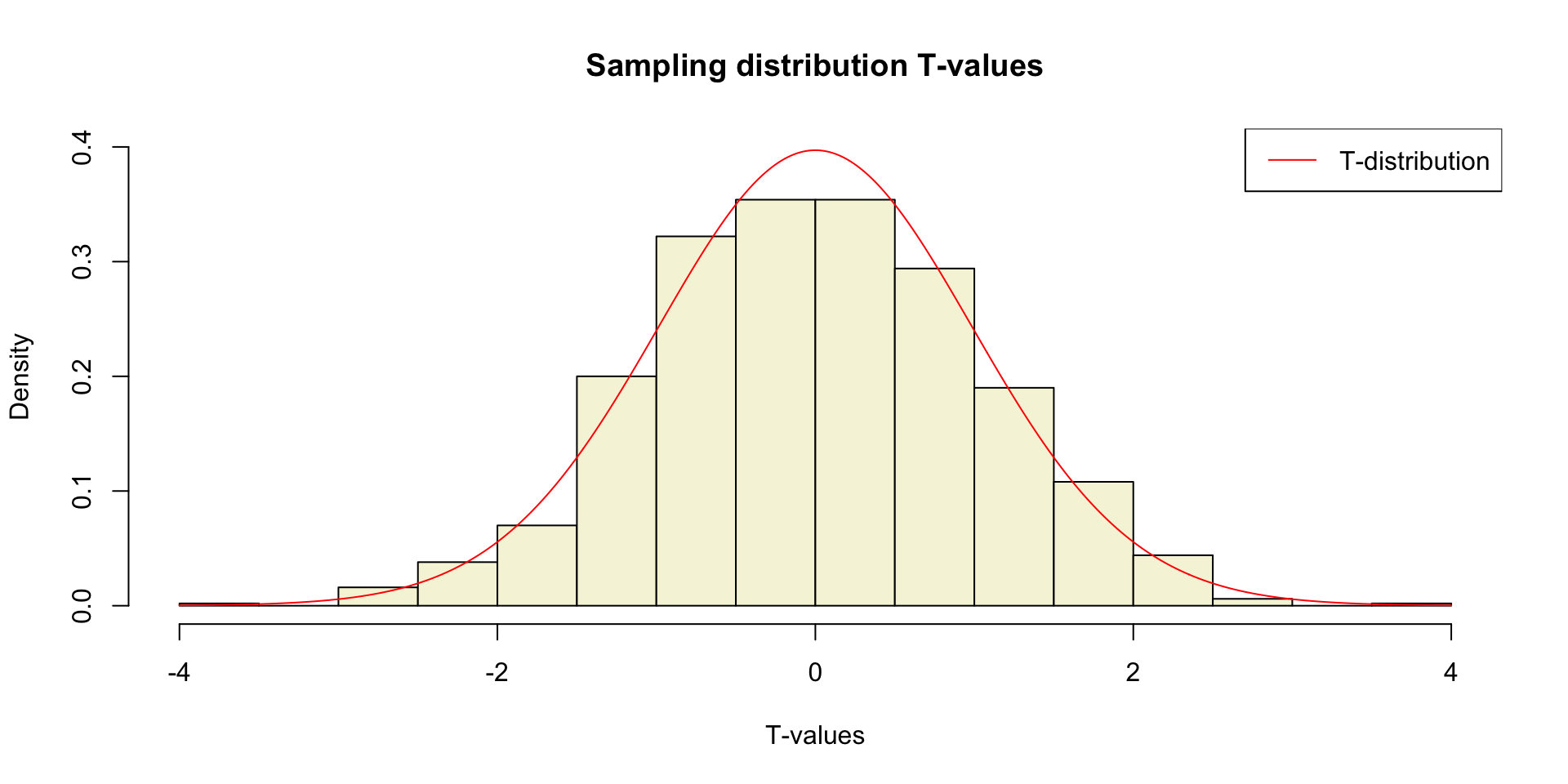
Sampling distribution t-values
Contact

References
Wikipedia. (2024). Student’s t-distribution — Wikipedia, the free encyclopedia. http://en.wikipedia.org/w/index.php?title=Student's%20t-distribution&oldid=1202978121.