F-distribution & Non-parametric tests

Author

Klinkenberg

Published

October 3, 2022

F-distribution

Ronald Fisher

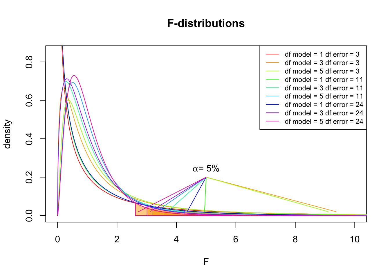
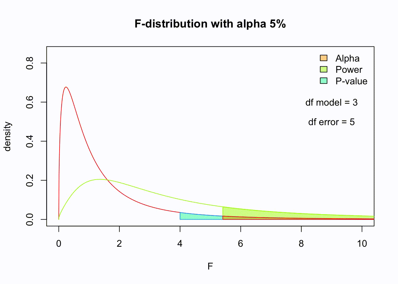
The F-distribution, also known as Snedecor’s F distribution or the Fisher–Snedecor distribution (after Ronald Fisher and George W. Snedecor) is, in probability theory and statistics, a continuous probability distribution. The F-distribution arises frequently as the null distribution of a test statistic, most notably in the analysis of variance; see F-test.

Wikipedia

Sir Ronald Aylmer Fisher FRS (17 February 1890 – 29 July 1962), known as R.A. Fisher, was an English statistician, evolutionary biologist, mathematician, geneticist, and eugenicist. Fisher is known as one of the three principal founders of population genetics, creating a mathematical and statistical basis for biology and uniting natural selection with Mendelian genetics.

Wikipedia

Ronald Fisher

Analysing variance

Decomposing variance example of height for males and females.

Population distribution

layout(matrix(c(2:6,1,1,7:8,1,1,9:13), 4, 4))

n  = 56    # Sample size
df = n - 1 # Degrees of freedom

mu    = 120
sigma = 15

IQ = seq(mu-45, mu+45, 1)

par(mar=c(4,2,0,0))  
plot(IQ, dnorm(IQ, mean = mu, sd = sigma), type='l', col="red")

n.samples = 12

for(i in 1:n.samples) {
  
  par(mar=c(2,2,0,0))  
  hist(rnorm(n, mu, sigma), main="", cex.axis=.5, col="red")
  
}

F-statistic

\[F = \frac{{MS}_{model}}{{MS}_{error}} = \frac{{SIGNAL}}{{NOISE}}\]

So the \(F\)-statistic represents a signal to noise ratio by deviding the model variance component by the error variance component.

A samples

Let’s take two sample from our normal populatiion and calculate the F-value.

x.1 = rnorm(n, mu, sigma)
x.2 = rnorm(n, mu, sigma)

data <- data.frame(group = rep(c("s1", "s2"), each=n), score = c(x.1,x.2))
    
F = summary(aov(lm(score ~ group, data)))[[1]]$F[1]
F
[1] 1.692487

More samples

let’s take more samples and calculate the F-value every time.

n.samples = 1000

f.values = vector()

for(i in 1:n.samples) {
  
  x.1 = rnorm(n, mu, sigma); x.1
  x.2 = rnorm(n, mu, sigma); x.2

  data <- data.frame(group = rep(c("s1", "s2"), each=n), score = c(x.1,x.2))
    
  f.values[i] = summary(aov(lm(score ~ group, data)))[[1]]$F[1]

}

k = 2
N = 2*n

df.model = k - 1
df.error = N - k

hist(f.values, freq = FALSE, main="F-values", breaks=100)
F = seq(0, 6, .01)
lines(F, df(F,df.model, df.error), col = "red")

F-distribution

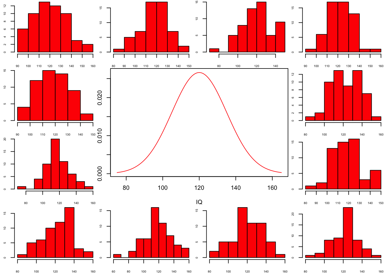
So if the population is normaly distributed (assumption of normality) the f-distribution represents the signal to noise ration given a certain number of samples (\({df}_{model} = k - 1\)) and sample size (\({df}_{error} = N - k\)).

The F-distibution therefore is different for different sample sizes and number of groups.

F-distribution

multiple.n  = c(5, 15, 30)
multiple.k  = c(2, 4, 6)
multiple.df.model = multiple.k - 1
multiple.df.error = multiple.n - multiple.k
col         = rainbow(length(multiple.df.model) * length(multiple.df.error))
F = seq(0, 10, .01)

plot(F,  df(F, multiple.df.model[1], multiple.df.error[1]), type = "l", 
     xlim = c(0,10), ylim = c(0,.85), 
     xlab = "F", ylab="density", 
     col  = col[1], main="F-distributions" )

dfs = expand.grid(multiple.df.model, multiple.df.error)

for(i in 2:dim(dfs)[1]) { 
  
  lines(F, df(F, dfs[i,1], dfs[i,2]), col=col[i])
  
  critical.f <- qf(.95, dfs[i,1], dfs[i,2])
  
  f.alpha <- seq(critical.f, 1000, .01)
  
  polygon(c(f.alpha, rev(f.alpha)), c(df(f.alpha, dfs[i,1], dfs[i,2]), f.alpha*0 ), col= rgb(1,.66,0, .5), border = col[i])
  
  lines(c(critical.f+.1, 5), c(.02, .2), col=col[i])
        
}

text(5,.2, expression(paste(alpha, "= 5%")), pos =3)

legend("topright", legend = paste("df model =",dfs[,1], "df error =", dfs[,2]), lty=1, col = col, cex=.75)

F-distribution

Animated F-distrigutions

Nonparametric tests

Parametric vs Nonparametric

Attribute Parametric Nonparametric
distribution normaly distributed any distribution
sampling random sample random sample
sensitivity to outliers yes no
works with large data sets small and large data sets
speed fast slow

Ranking

x = c(1, 4, 6, 7, 8, 9)
y = c(1, 4, 6, 7, 8, 39)

layout(matrix(1:2, 1, 2))
boxplot(x, horizontal=T, col='red')
boxplot(y, horizontal=T, col='red')

kable(rbind(rx = rank(x), ry = rank(y)))
rx 1 2 3 4 5 6
ry 1 2 3 4 5 6

Ties

# Scores
x = c(11, 42, 62, 73, 84, 84, 42, 73, 90); x
[1] 11 42 62 73 84 84 42 73 90
# sort
sort(x)
[1] 11 42 42 62 73 73 84 84 90
# assign ranks
1:length(x)
[1] 1 2 3 4 5 6 7 8 9
# solve for ties
rank(sort(x))
[1] 1.0 2.5 2.5 4.0 5.5 5.5 7.5 7.5 9.0

\[\frac{2 + 3}{2} = 2.5, \frac{5 + 6}{2} = 5.5, \frac{7 + 8}{2} = 7.5\]

Procedure

  1. Assumption: independent random samples.
  2. Hypothesis:
    \(H_0\) : equal population distributions (implies equal mean ranking)
    \(H_A\) : unequal mean ranking (two sided)
    \(H_A\) : higher mean ranking for one group.
  3. Test statistic is difference between mean or sum of ranking.
  4. Standardise test statistic
  5. Calculate P-value one or two sided.
  6. Conclude to reject \(H_0\) if \(p < \alpha\).

Kruskal–Wallis test

Independent >2 samples

Kruskal–Wallis test

Created by William Henry Kruskal (L) and Wilson Allen Wallis (R), the Kruskal-Wallis test is a nonparametric alternative to the independent one-way ANOVA.

The Kruskal-Wallis test essentially subtracts the expected mean ranking from the calculated oberved mean ranking, which is \(\chi^2\) distributed.

Simulate data

n      = 30
factor = rep(c("ecstasy","alcohol","control"), each=n/3)

dummy.1 = ifelse(factor == "alcohol", 1, 0)
dummy.2 = ifelse(factor == "ecstasy", 1, 0)
b.0     = 23
b.1     = 0
b.2     = 0
error   = rnorm(n, 0, 1.7)

# Model
depres  = b.0 + b.1*dummy.1 + b.2*dummy.2 + error
depres  = round(depres)

data <- data.frame(factor, depres)

Assign ranks

# Assign ranks
data$ranks = rank(data$depres)

The data

Calculate H

\[H = \frac{12}{N(N+1)} \sum_{i=1}^k \frac{R_i^2}{n_i} - 3(N+1)\]

  • \(N\) total sample size
  • \(n_i\) sample size per group
  • \(k\) number of groups
  • \(R_i\) rank sums per group

Calculate H

# Now we need the sum of the ranks per group.
R.i = aggregate(ranks ~ factor, data = data, sum)$ranks
R.i
[1] 207.0 121.5 136.5
# De total sample size N is:
N = nrow(data)

# And the sample size per group is n_i:
n.i = aggregate(depres ~ factor, data=data, length)$depres
n.i
[1] 10 10 10

Calculate H

\[H = \frac{12}{N(N+1)} \sum_{i=1}^k \frac{R_i^2}{n_i} - 3(N+1)\]

H = ( 12/(N*(N+1)) ) * sum(R.i^2/n.i) - 3*(N+1)
H
[1] 5.37871

And the degrees of freedom

k  = 3
df = k - 1

Test for significance

visualize.chisq(H, df, section="upper")

End

Contact

CC BY-NC-SA 4.0