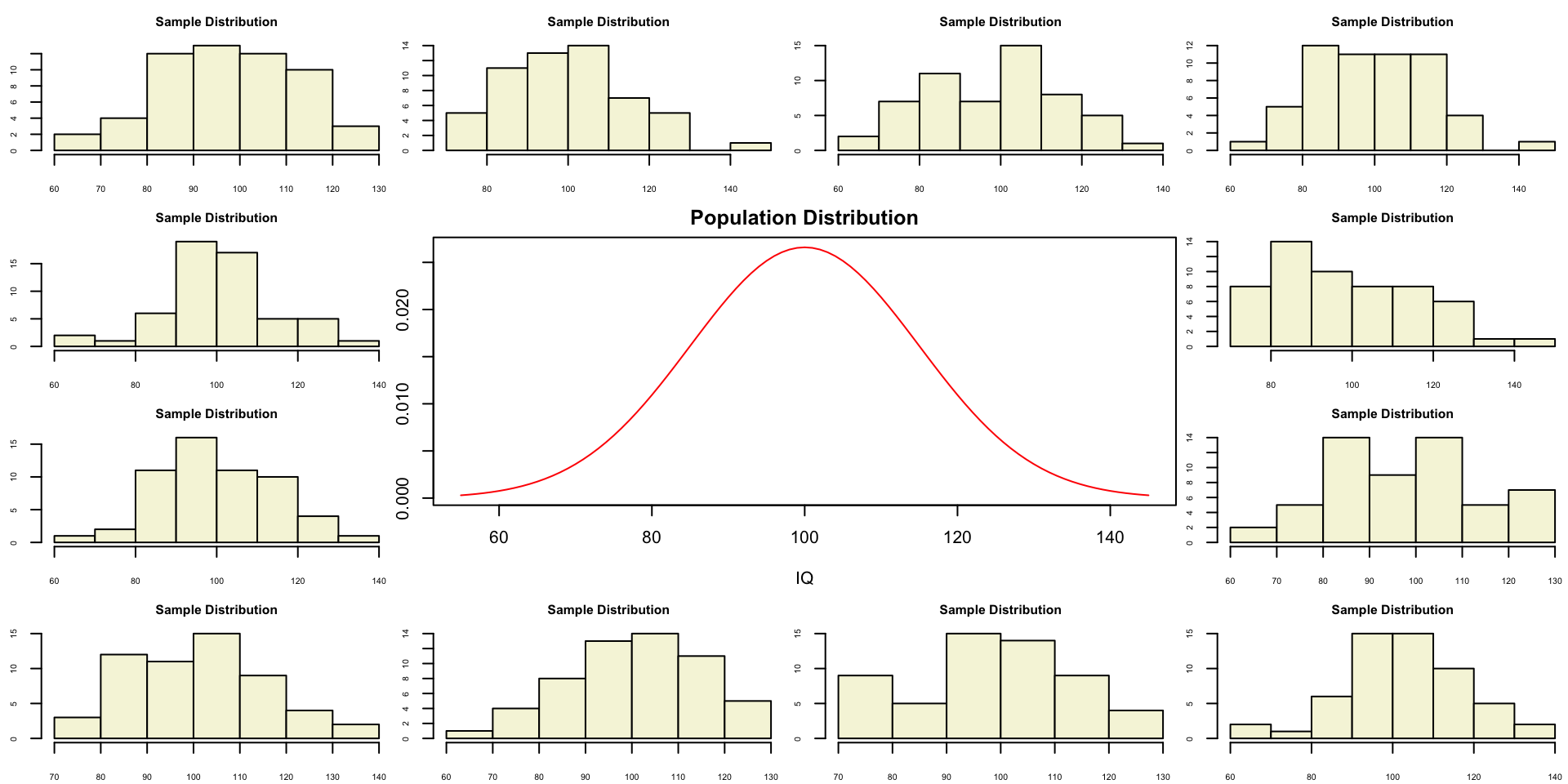
layout(matrix(c(2:6,1,1,7:8,1,1,9:13), 4, 4))

n  = 56    # Sample size
df = n - 1 # Degrees of freedom

mu    = 100
sigma = 15

IQ = seq(mu-45, mu+45, 1)

par(mar=c(4,2,2,0))
plot(IQ, dnorm(IQ, mean = mu, sd = sigma), type='l', col="red", main = "Population Distribution")

n.samples = 12

for(i in 1:n.samples) {

  par(mar=c(2,2,2,0))
  hist(rnorm(n, mu, sigma), main="Sample Distribution", cex.axis=.5, col="beige", cex.main = .75)

}T-distribution and the
One-sample t-test
Klinkenberg
University of Amsterdam
20 sep 2022
T-distribution
Gosset

In probability and statistics, Student’s t-distribution (or simply the t-distribution) is any member of a family of continuous probability distributions that arises when estimating the mean of a normally distributed population in situations where the sample size is small and population standard deviation is unknown.
In the English-language literature it takes its name from William Sealy Gosset’s 1908 paper in Biometrika under the pseudonym “Student”. Gosset worked at the Guinness Brewery in Dublin, Ireland, and was interested in the problems of small samples, for example the chemical properties of barley where sample sizes might be as low as 3.
Source: Wikipedia
Population distribution
Population distribution
A sample
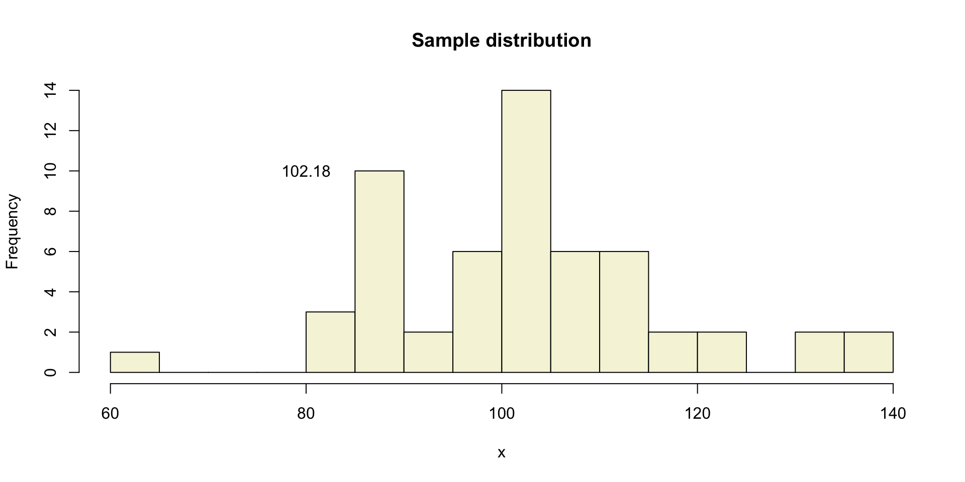
Let’s take one sample from our normal populatiion and calculate the t-value.
 [1]  90.29226  86.50468  82.67459  87.52014 109.47630  98.08283  87.67426
 [8] 104.11862  90.84647 102.19677 109.45225 108.74995 137.29301 104.96585
[15]  85.70202 100.49200  86.03716  87.62016 104.32542  98.36916 112.92071
[22]  96.43524  81.46636 111.04604 114.71462 135.98574  97.31552 100.96565
[29] 113.32101 101.34637  87.97518 102.77408 122.15193 103.17731  86.67964
[36] 105.05558 122.54113 117.60647 111.24434 101.70309 130.46728  98.23638
[43] 111.14123 104.96811  97.33341 100.28260  85.72114 107.43696 101.52655
[50] 101.63470 108.97211 117.24962 82.24049 87.62497 134.93508 63.65653A sample
More samples
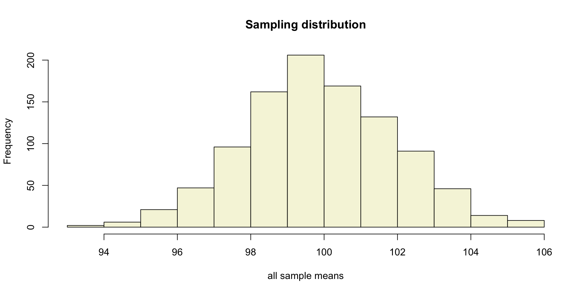
let’s take more samples.
Mean and SE for all samples
Sampling distribution
Of the mean
Sampling distribution
T-statistic
\[T_{n-1} = \frac{\bar{x}-\mu}{SE_x} = \frac{\bar{x}-\mu}{s_x / \sqrt{n}}\]
So the t-statistic represents the deviation of the sample mean \(\bar{x}\) from the population mean \(\mu\), considering the sample size, expressed as the degrees of freedom \(df = n - 1\)
t-value
\[T_{n-1} = \frac{\bar{x}-\mu}{SE_x} = \frac{\bar{x}-\mu}{s_x / \sqrt{n}}\]
Calculate t-values
\[T_{n-1} = \frac{\bar{x}-\mu}{SE_x} = \frac{\bar{x}-\mu}{s_x / \sqrt{n}}\]
        mean.x.values  mu se.x.values   t.values
 [995,]     102.68990 100    2.151975  1.2499683
 [996,]      98.13215 100    2.102059 -0.8885817
 [997,]      98.31403 100    1.927675 -0.8746117
 [998,]      95.94184 100    2.087404 -1.9441195
 [999,]     104.30809 100    1.918401  2.2456652
[1000,]      99.41000 100    2.099974 -0.2809564
Sampled t-values
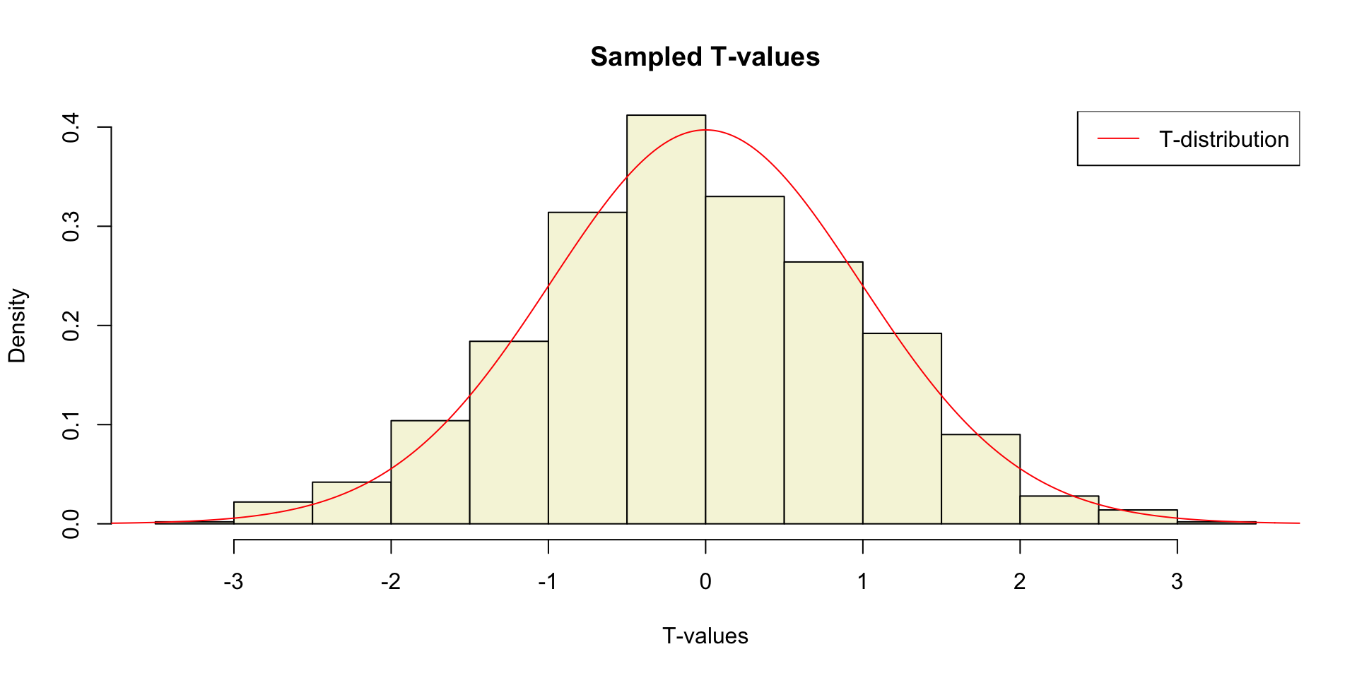
What is the distribution of all these t-values?
Sampled t-values
T-distribution
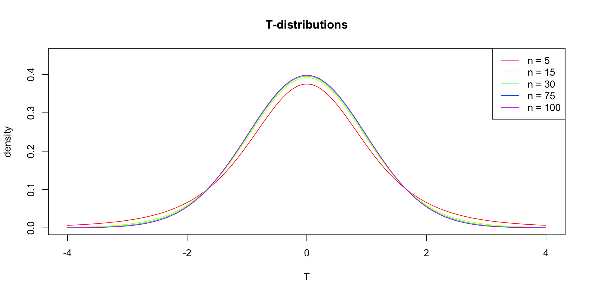
So if the population is normaly distributed (assumption of normality) the t-distribution represents the deviation of sample means from the population mean (\(\mu\)), given a certain sample size (\(df = n - 1\)).
The t-distibution therefore is different for different sample sizes and converges to a standard normal distribution if sample size is large enough.
The t-distribution is defined by:
\[\textstyle\frac{\Gamma \left(\frac{\nu+1}{2} \right)} {\sqrt{\nu\pi}\,\Gamma \left(\frac{\nu}{2} \right)} \left(1+\frac{x^2}{\nu} \right)^{-\frac{\nu+1}{2}}\!\]
where \(\nu\) is the number of degrees of freedom and \(\Gamma\) is the gamma function.
Source: wikipedia
One or two sided
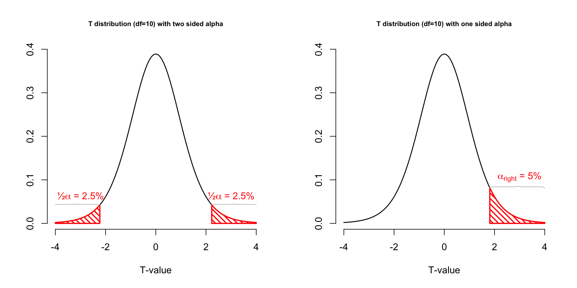
Two sided
- \(H_A: \bar{x} \neq \mu\)
One sided
- \(H_A: \bar{x} > \mu\)
- \(H_A: \bar{x} < \mu\)
Effect-size
The effect-size is the standardised difference between the mean and the expected \(\mu\). In the t-test effect-size is expressed as \(r\).
\[r = \sqrt{\frac{t^2}{t^2 + \text{df}}}\]
Effect-sizes
We can also calculate effect-sizes for all our calculated t-values. Under the assumption of \(H_0\) the effect-size distribution looks like this.
        mean.x.values  mu se.x.values   t.values         r
 [995,]     102.68990 100    2.151975  1.2499683 0.1662015
 [996,]      98.13215 100    2.102059 -0.8885817 0.1189654
 [997,]      98.31403 100    1.927675 -0.8746117 0.1171210
 [998,]      95.94184 100    2.087404 -1.9441195 0.2535769
 [999,]     104.30809 100    1.918401  2.2456652 0.2898103
[1000,]      99.41000 100    2.099974 -0.2809564 0.0378570
Effect-size distribution

Cohen (1988)
- Small: \(0 \leq .1\)
- Medium: \(.1 \leq .3\)
- Large: \(.3 \leq .5\)
Power
- Strive for 80%
- Based on know effect size
- Calculate number of subjects needed
- Use G*Power to calculate
Alpha Power
T = seq(-3,6,.01)
N = 45
E = 2

# Set plot
plot(0,0,
     type = "n",
     ylab = "Density",
     xlab = "T",
     ylim = c(0,.5),
     xlim = c(-3,6),
     main = "T-Distributions under H0 and HA")

critical_t = qt(.05,N-1,lower.tail=FALSE)

# Alpha
range_x = seq(critical_t,6,.01)
polygon(c(range_x,rev(range_x)),
        c(range_x*0,rev(dt(range_x,N-1,ncp=0))),
        col     = "grey",
        density = 10,
        angle   = 90,
        lwd     = 2)

# Power
range_x = seq(critical_t,6,.01)
polygon(c(range_x,rev(range_x)),
        c(range_x*0,rev(dt(range_x,N-1,ncp=E))),
        col     = "grey",
        density = 10,
        angle   = 45,
        lwd     = 2)

lines(T,dt(T,N-1,ncp=0),col="red", lwd=2) # H0 line
lines(T,dt(T,N-1,ncp=E),col="blue",lwd=2) # HA line

# Critical value
lines(rep(critical_t,2),c(0,dt(critical_t,N-1,ncp=E)),lwd=2,col="black")
text(critical_t,dt(critical_t,N-1,ncp=E),"critical T-value",pos=2, srt = 90)

# H0 and HA
text(0,dt(0,N-1,ncp=0),expression(H[0]),pos=3,col="red", cex=2)
text(E,dt(E,N-1,ncp=E),expression(H[A]),pos=3,col="blue",cex=2)

# Mu H0 line
lines(c(0,0),c(0,dt(0,N-1)), col="red",  lwd=2,lty=2)
text(0,dt(0,N-1,ncp=0)/2,expression(mu),pos=4,cex=1.2)
# Mu HA line
lines(c(E,E),c(0,dt(E,N-1,ncp=E)),col="blue",lwd=2,lty=2)
text(E,dt(0,N-1,ncp=0)/2,expression(paste(mu)),pos=4,cex=1.2)

# t-value
lines( c(critical_t+.01,6),c(0,0),col="green",lwd=4)

# Legend
legend("topright", c(expression(alpha),'POWER'),density=c(10,10),angle=c(90,45))
Alpha Power

One-sample t-test
IQ next to you

http://goo.gl/T6Lo2s
Models
\[\text{outcome} = \text{model} + \text{error}\]
Compare sample mean
We use the one-sample t-test to compare the sample mean \(\bar{x}\) to the population mean \(\mu\).
Let’s take a different sample and calculate the mean of this sample.
mu     = 120
n      = length(IQ.next.to.you)
x      = IQ.next.to.you
mean_x = mean(x, na.rm = TRUE)
sd_x   = sd(x, na.rm = TRUE)
cbind(n, mean_x, sd_x)
n mean_x sd_x
[1,] 77 119.9091 12.71673Does this mean, differ significantly from the population mean \(\mu = 120\)?
Hypothesis
Null hypothesis
- \(H_0: \bar{x} = \mu\)
Alternative hypothesis
- \(H_A: \bar{x} \neq \mu\)
- \(H_A: \bar{x} > \mu\)
- \(H_A: \bar{x} < \mu\)
Assumptions
- Normal samples distribution
- Random sample
- Measurement level
- Interval
- Ratio
T-statistic
\[T_{n-1} = \frac{\bar{x}-\mu}{SE_x} = \frac{\bar{x}-\mu}{s_x / \sqrt{n}} = \frac{119.91 - 120 }{12.72 / \sqrt{77}}\]
So the t-statistic represents the deviation of the sample mean \(\bar{x}\) from the population mean \(\mu\), considering the sample size.
Type I error
To determine if this t-value significantly differs from the population mean we have to specify a type I error that we are willing to make.
- Type I error / \(\alpha\) = .05
P-value one sided
Finally we have to calculate our p-value for which we need the degrees of freedom \(df = n - 1\) to determine the shape of the t-distribution.
P-value one sided

P-value two sided

Effect-size
\[r = \sqrt{\frac{t^2}{t^2 + \text{df}}}\]
End
Contact

Scientific & Statistical Reasoning
