William Sealy Gosset (aka Student) in 1908 (age 32)
In probability and statistics, Student’s t-distribution (or simply the t-distribution) is any member of a family of continuous probability distributions that arises when estimating the mean of a normally distributed population in situations where the sample size is small and population standard deviation is unknown.
In the English-language literature it takes its name from William Sealy Gosset’s 1908 paper in Biometrika under the pseudonym “Student”. Gosset worked at the Guinness Brewery in Dublin, Ireland, and was interested in the problems of small samples, for example the chemical properties of barley where sample sizes might be as low as 3.
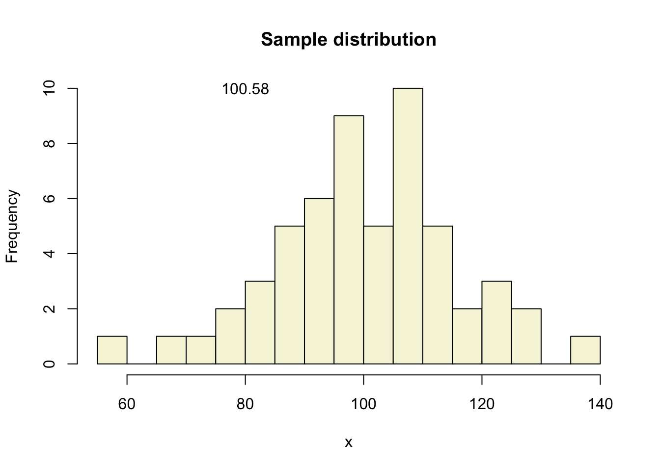
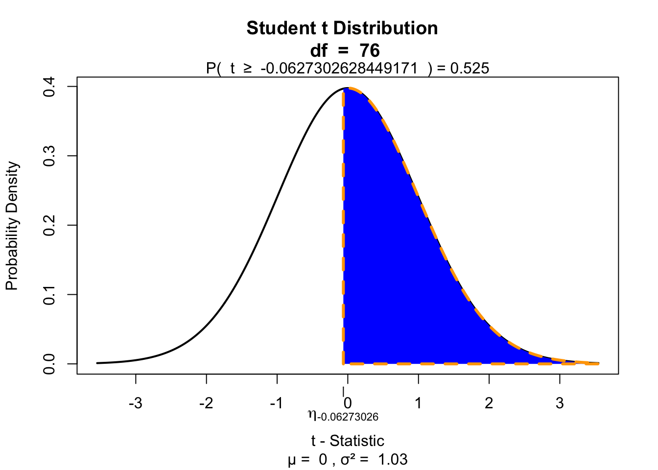
So the t-statistic represents the deviation of the sample mean \(\bar{x}\) from the population mean \(\mu\), considering the sample size, expressed as the degrees of freedom \(df = n - 1\)
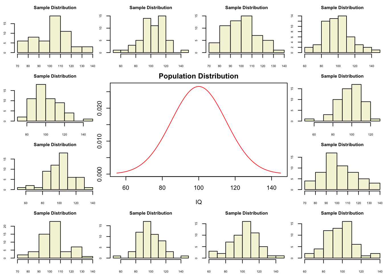
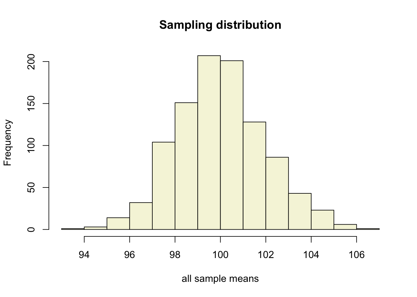
So if the population is normaly distributed (assumption of normality) the t-distribution represents the deviation of sample means from the population mean (\(\mu\)), given a certain sample size (\(df = n - 1\)).
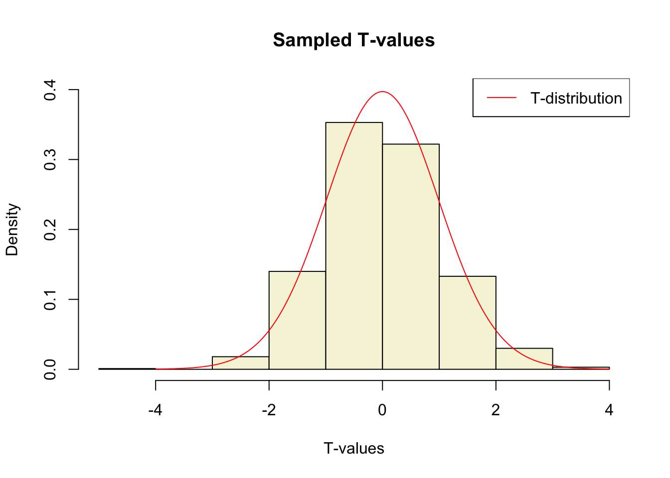
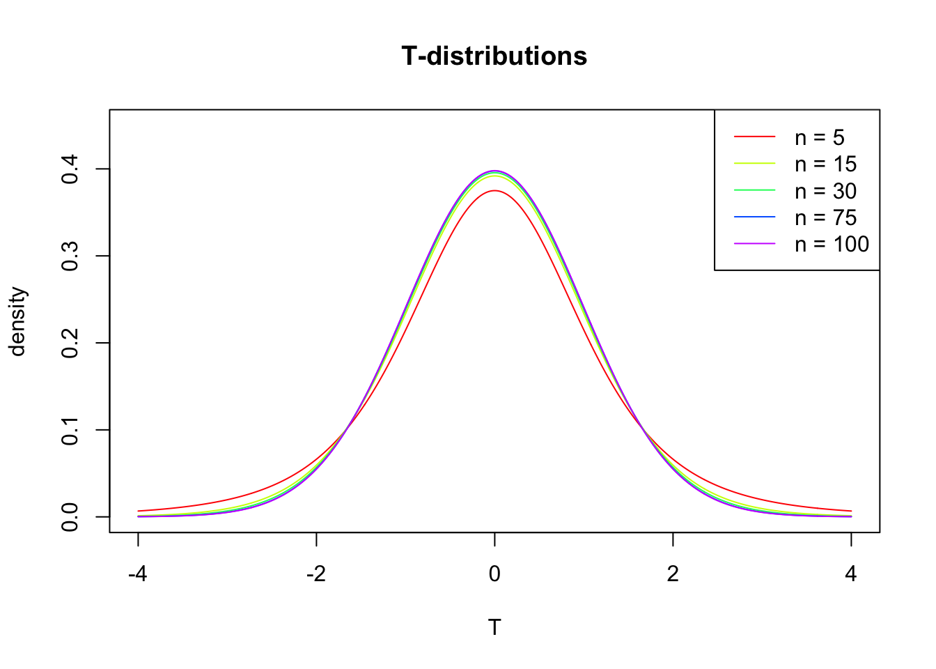
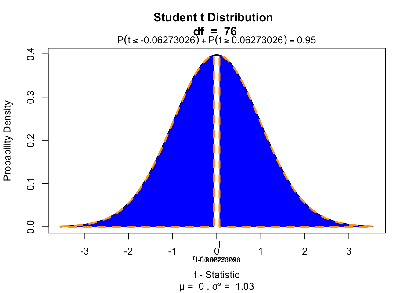
The t-distibution therefore is different for different sample sizes and converges to a standard normal distribution if sample size is large enough.