Non-parametric tests

Klinkenberg

University of Amsterdam

7 oct 2022

Nonparametric tests

Parametric vs Nonparametric

Attribute	Parametric	Nonparametric
distribution	normaly distributed	any distribution
sampling	random sample	random sample
sensitivity to outliers	yes	no
works with	large data sets	small and large data sets
speed	fast	slow

Ranking

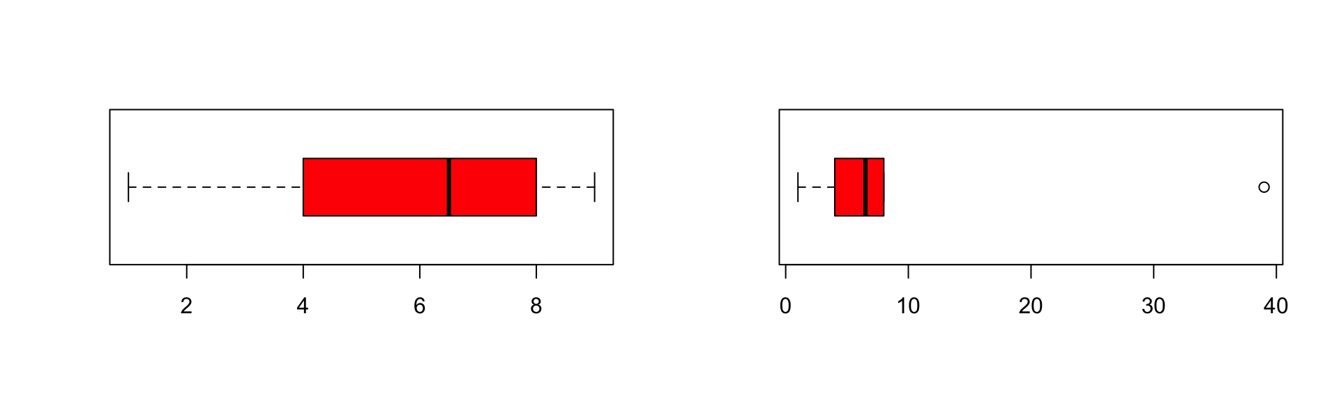
rx	1	2	3	4	5	6
ry	1	2	3	4	5	6

Ties

# Scores
x = c(11, 42, 62, 73, 84, 84, 42, 73, 90)

# sort
order = sort(x)

# assign ranks
ranks = 1:length(x)

# solve for ties
ties = rank(sort(x))

x	11	42.0	62.0	73	84.0	84.0	42.0	73.0	90
order	11	42.0	42.0	62	73.0	73.0	84.0	84.0	90
ranks	1	2.0	3.0	4	5.0	6.0	7.0	8.0	9
ties	1	2.5	2.5	4	5.5	5.5	7.5	7.5	9

\[\frac{2 + 3}{2} = 2.5, \frac{5 + 6}{2} = 5.5, \frac{7 + 8}{2} = 7.5\]

Procedure

Assumption: independent random samples.
Hypothesis:
\(H_0\) : equal population distributions (implies equal mean ranking)
\(H_A\) : unequal mean ranking (two sided)
\(H_A\) : higher mean ranking for one group.
Test statistic is difference between mean or sum of ranking.
Standardise test statistic
Calculate P-value one or two sided.
Conclude to reject \(H_0\) if \(p < \alpha\).

Wilcoxon rank-sum test

Independent 2 samples

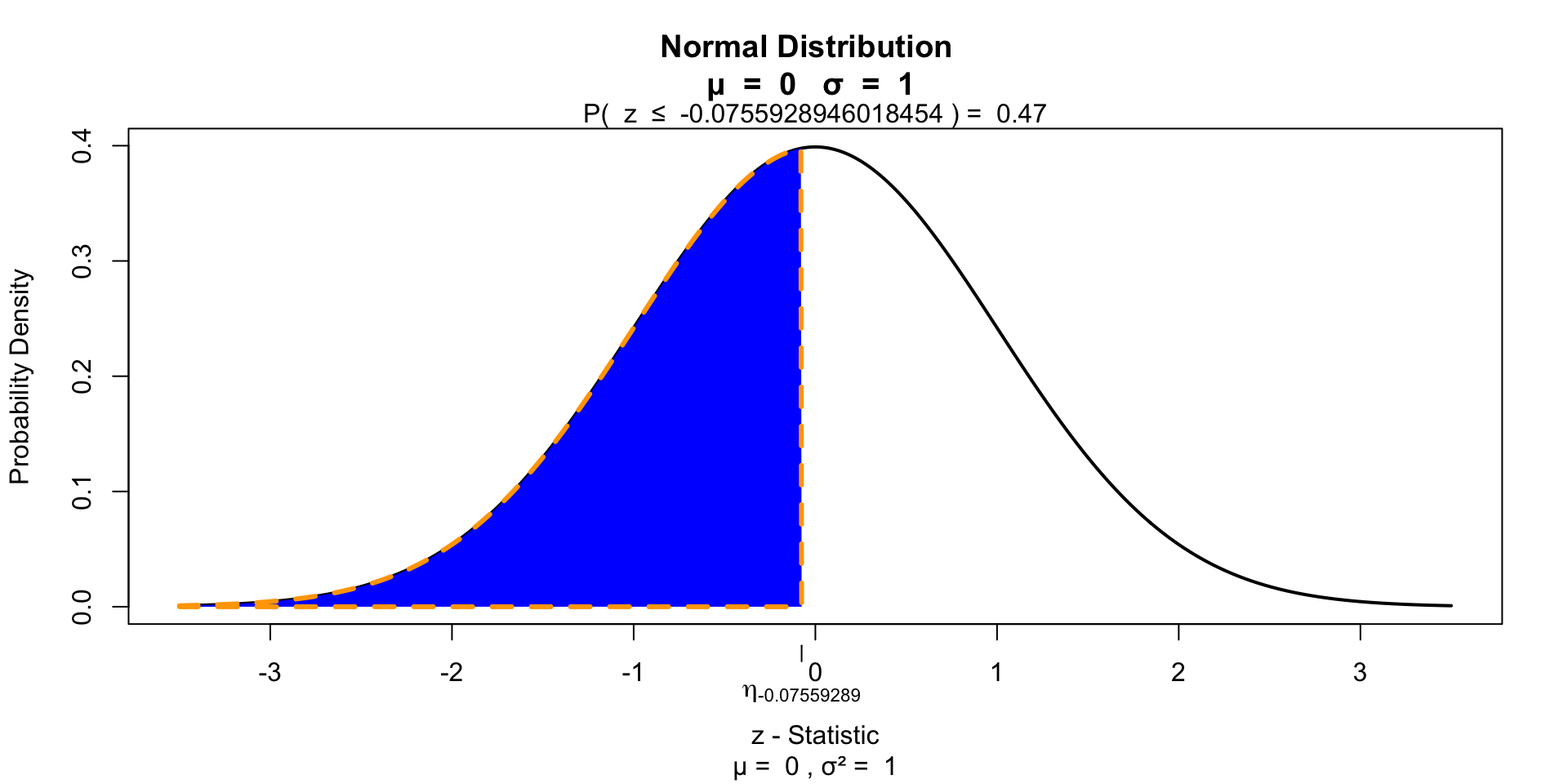
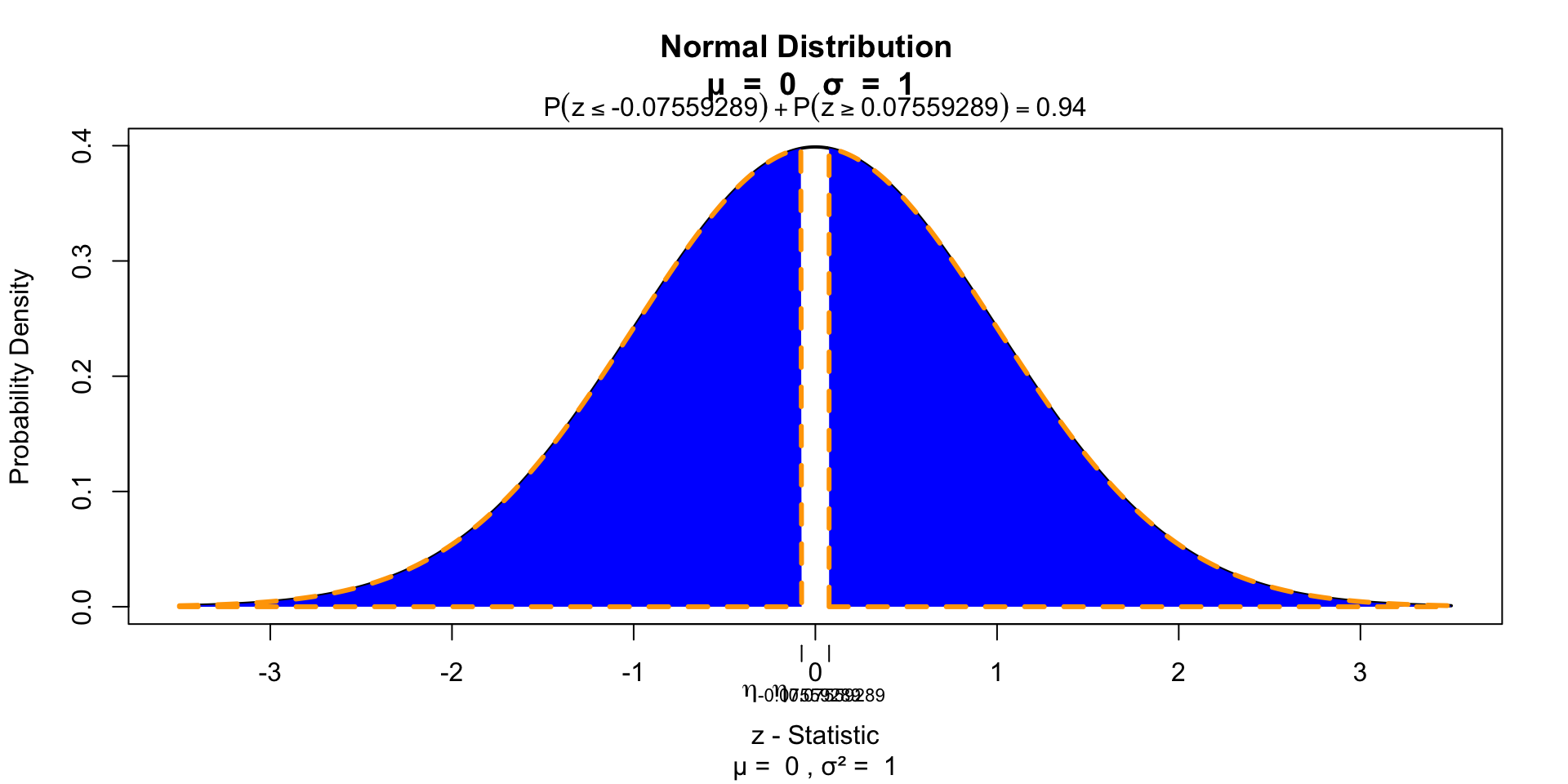
Wilcoxon rank-sum test

Developed by Frank Wilcoxon the rank-sum test is a nonparametric alternative to the independent samples t-test.

By first ranking \(x\) and then sum these ranks per group one would expect, under the null hypothesis, equal values for both groups.

After standardising this difference one can test using a standard normal distribution.

Sum the ranks

Sum the ranks example for height for males and females.

Simulate data

n      = 20
factor = rep(c("Ecstasy","Alcohol"),each=n/2)
dummy  = ifelse(factor == "Ecstacy", 0, 1)
b.0    = 23
b.1    = 5
error  = rnorm(n, 0, 1.7)
depres = b.0 + b.1*dummy + error
depres = round(depres)

data <- data.frame(factor, depres)

## add the ranks
data$R <- rank(data$depres)

Example

Calculate the sum of ranks per group

R <- aggregate(R ~ factor, data, sum)
R

   factor   R
1 Alcohol 104
2 Ecstasy 106

So W is the lowest

\[W=min\left(\sum{R_1},\sum{R_2}\right)\]

W <- min(R$R)
W

[1] 104

Standardise W

To calculate the Z score we need to standardise the W. To do so we need the mean W and the standard error of W.

For this we need the sample sizes for each group.

n <- aggregate(R ~ factor, data, length)

n.1 = n$R[1]
n.2 = n$R[2]

cbind(n.1, n.2)

     n.1 n.2
[1,]  10  10

Mean W

\[\bar{W}_s=\frac{n_1(n_1+n_2+1)}{2}\]

W.mean = (n.1*(n.1+n.2+1))/2
W.mean

[1] 105

SE W

\[{SE}_{\bar{W}_s}=\sqrt{ \frac{n_1 n_2 (n_1+n_2+1)}{12} }\]

W.se = sqrt((n.1*n.2*(n.1+n.2+1))/12)
W.se

[1] 13.22876

Calculate Z

\[z = \frac{W - \bar{W}}{{SE}_W}\]

Which looks a lot like

\[\frac{X - \bar{X}}{{SE}_X} \text{or} \frac{b - \mu_{b}}{{SE}_b} \]

z = (W - W.mean) / W.se
z

[1] -0.07559289

Test for significance 1 sided

if(!"visualize" %in% installed.packages()){ install.packages("visualize") }
library("visualize")

visualize.norm(z, section="lower")

Test for significance 2 sided

visualize.norm(c(z,-z), section="tails")

Effect size

\[r = \frac{z}{\sqrt{N}}\]

N = sum(n$R)
r = z / sqrt(N)
r

[1] -0.01690309

Mann–Whitney test

\[U = n_1 n_2 + \frac{n_1 (n_1 + 1)}{2} - R_1\]

U = (n.1*n.2)+(n.1*(n.1+1))/2-R$R[1]
U

[1] 51

\(\bar{U}\) and \({SE}_U\) for non tied ranks

\[\bar{U} = \frac{n_1 n_2}{2}\]

(n.1*n.2)/2

[1] 50

\[{SE}_U = \sqrt{\frac{n_1 n_2 (n_1 + n_2 + 1)}{12}}\]

sqrt((n.1*n.2*(n.1+n.2+1))/12)

[1] 13.22876

Wilcoxon signed-rank test

Paired 2 samples

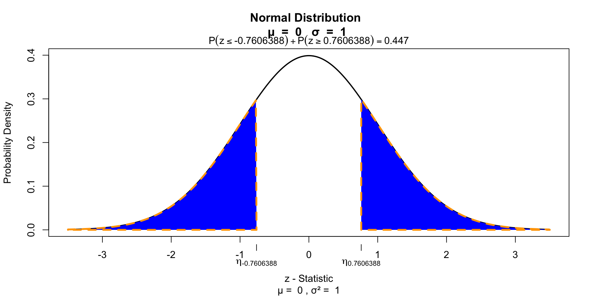
Wilcoxon signed-rank test

The Wilcoxon signed-rank test is a nonparametric alternative to the paired samples t-test. It assigns + or - signs to the difference between two repeated measures. By ranking the differences and summing these ranks for the positive group, the null hypothesis is tested that both positive and negative differences are equal.

Simulate data

n      = 20
factor = rep(c("Ecstasy","Alcohol"),each=n/2)
dummy  = ifelse(factor == "Ecstacy", 0, 1)
b.0    = 23
b.1    = 5
error  = rnorm(n, 0, 1.7)
depres = b.0 + b.1*dummy + error
depres = round(depres)

data <- data.frame(factor, depres)

Ecstasy <- subset(data, factor=="Ecstasy")$depres
Alcohol <- subset(data, factor=="Alcohol")$depres

data <- data.frame(Ecstasy, Alcohol)

Example

Calculate T

# Calculate difference in scores between first and second measure
data$difference = data$Ecstasy - data$Alcohol

# Calculate absolute difference in scores between first and second measure
data$abs.difference = abs(data$Ecstasy - data$Alcohol)

# Create rank variable with place holder NA
data$rank <- NA

# Rank only the difference scores
data[which(data$difference != 0),'rank'] <- rank(data[which(data$difference != 0),
                                                      'abs.difference'])

# Assign a '+' or a '-' to those values 
data$sign = sign(data$Ecstasy - data$Alcohol)

# Add positive and negative rank to     test  if    else
data$rank_pos = with(data, ifelse(sign ==  1, rank, 0   ))
data$rank_neg = with(data, ifelse(sign == -1, rank, 0   ))

The data

Calculate \(T_+\)

# Calculate the sum of the positive ranks
T_pos = sum(data$rank_pos)
T_pos

[1] 18.5

# Calculate N without 0 (no differences).
n = sum(abs(data$sign))
n

[1] 7

Calculate \(\bar{T}\) and \({SE}_{T}\)

\[\bar{T} = \frac{n(n+1)}{4}\]

T_mean = (n*(n+1))/4
T_mean

[1] 14

\[{SE}_{T} = \sqrt{\frac{n(n+1)(2n+1)}{24}}\]

SE_T = sqrt( (n*(n+1)*(2*n+1)) / 24 )

Calculate Z

\[z = \frac{T_+ - \bar{T}}{{SE}_T}\]

z = (T_pos - T_mean)/SE_T
z

[1] 0.7606388

Test for significance

visualize.norm(c(z,-z), section="tails")

Effect size

\[r = \frac{z}{\sqrt{N}}\]

Here \(N\) is the number of observations.

N = 20
r = z / sqrt(N)
r

[1] 0.170084

Kruskal–Wallis test

Independent >2 samples

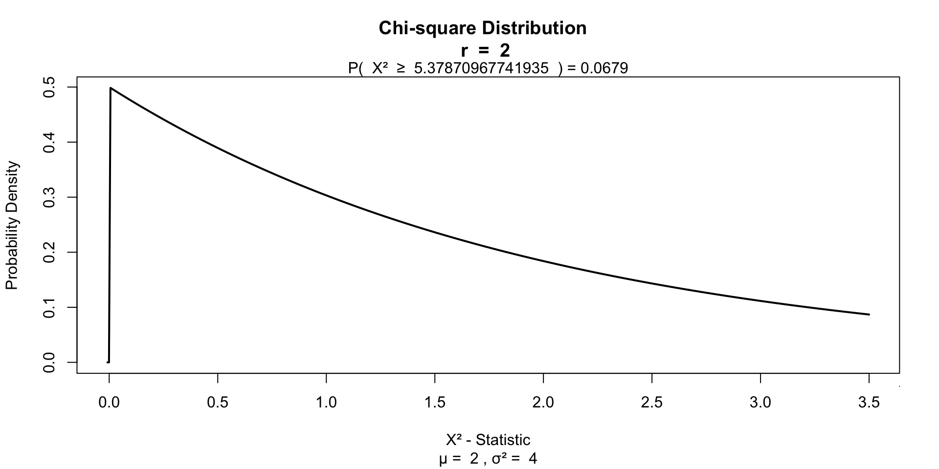
Kruskal–Wallis test

Created by William Henry Kruskal (L) and Wilson Allen Wallis (R), the Kruskal-Wallis test is a nonparametric alternative to the independent one-way ANOVA.

The Kruskal-Wallis test essentially subtracts the expected mean ranking from the calculated oberved mean ranking, which is \(\chi^2\) distributed.

Simulate data

n      = 30
factor = rep(c("ecstasy","alcohol","control"), each=n/3)

dummy.1 = ifelse(factor == "alcohol", 1, 0)
dummy.2 = ifelse(factor == "ecstasy", 1, 0)
b.0     = 23
b.1     = 0
b.2     = 0
error   = rnorm(n, 0, 1.7)

# Model
depres  = b.0 + b.1*dummy.1 + b.2*dummy.2 + error
depres  = round(depres)

data <- data.frame(factor, depres)

Assign ranks

# Assign ranks
data$ranks = rank(data$depres)

The data

Calculate H

\[H = \frac{12}{N(N+1)} \sum_{i=1}^k \frac{R_i^2}{n_i} - 3(N+1)\]

\(N\) total sample size
\(n_i\) sample size per group
\(k\) number of groups
\(R_i\) rank sums per group

Calculate H

# Now we need the sum of the ranks per group.
R.i = aggregate(ranks ~ factor, data = data, sum)$ranks
R.i

[1] 207.0 121.5 136.5

# De total sample size N is:
N = nrow(data)

# And the sample size per group is n_i:
n.i = aggregate(depres ~ factor, data=data, length)$depres
n.i

[1] 10 10 10

Calculate H

\[H = \frac{12}{N(N+1)} \sum_{i=1}^k \frac{R_i^2}{n_i} - 3(N+1)\]

H = ( 12/(N*(N+1)) ) * sum(R.i^2/n.i) - 3*(N+1)
H

[1] 5.37871

And the degrees of freedom

k  = 3
df = k - 1

Test for significance

visualize.chisq(H, df, section="upper")

Friedman’s ANOVA

Paired >2 samples

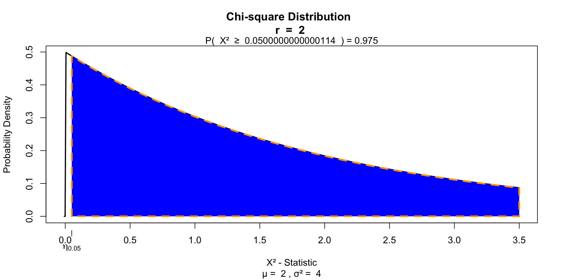
Friedman’s ANOVA

Created by William Frederick Friedman the Friedman’s ANOVA is a nonparametric alternative to the repeated one-way ANOVA.

Just like the Kruskal-Wallis test, Friedman’s ANOVA, subtracts the expected mean ranking from the calculated observed mean ranking, which is also \(\chi^2\) distributed.

Simulate data

n      = 30
factor = rep(c("ecstasy","alcohol","control"), each=n/3)

dummy.1 = ifelse(factor == "alcohol", 1, 0)
dummy.2 = ifelse(factor == "ecstasy", 1, 0)
b.0     = 23
b.1     = 0
b.2     = 0
error   = rnorm(n, 0, 1.7)

# Model
depres  = b.0 + b.1*dummy.1 + b.2*dummy.2 + error
depres  = round(depres)

data <- data.frame(factor, depres)

Simulate data

ecstasy <- subset(data, factor=="ecstasy")$depres
alcohol <- subset(data, factor=="alcohol")$depres
control <- subset(data, factor=="control")$depres

data <- data.frame(ecstasy, alcohol, control)

The data

Assign ranks

Rank each row.

# Rank for each person
ranks = t(apply(data, 1, rank))

The data with ranks

Calculate \(F_r\)

\[F_r = \left[ \frac{12}{Nk(k+1)} \sum_{i=1}^k R_i^2 \right] - 3N(k+1)\]

\(N\) total number of subjects
\(k\) number of groups
\(R_i\) rank sums for each group

Calculate \(F_r\)

Calculate ranks sum per condition and \(N\).

R.i = apply(ranks, 2, sum)
R.i

ecstasy alcohol control 
   20.0    19.5    20.5

# N is number of participants
N = 10

Calculate \(F_r\)

\[F_r = \left[ \frac{12}{Nk(k+1)} \sum_{i=1}^k R_i^2 \right] - 3N(k+1)\]

k = 3
F.r = ( ( 12/(N*k*(k+1)) ) * sum(R.i^2) ) - ( 3*N*(k+1) )
F.r

[1] 0.05

And the degrees of freedom

df = k - 1

Test for significance

visualize.chisq(F.r, df, section="upper")

End

Contact