Multiple regression

Klinkenberg

University of Amsterdam

10 nov 2022

Multiple regression

\(\LARGE{\text{outcome} = \text{model} + \text{error}}\)

In statistics, linear regression is a linear approach for modeling the relationship between a scalar dependent variable y and one or more explanatory variables denoted X.

\(\LARGE{Y_i = \beta_0 + \beta_1 X_{1i} + \beta_2 X_{2i} + \dotso + \beta_n X_{ni} + \epsilon_i}\)

In linear regression, the relationships are modeled using linear predictor functions whose unknown model parameters \(\beta\)’s are estimated from the data.

Source: wikipedia

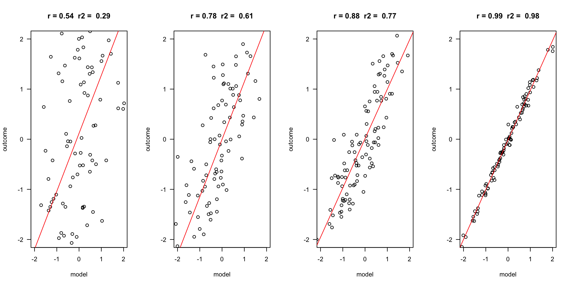
Outcome vs Model

Assumptions

A selection from Field (8.3.2.1. Assumptions of the linear model):

For simple regression

Sensitivity
Homoscedasticity

For multiple regressin

Multicollinearity
Linearity

Multicollinearity

To adhere to the multicollinearity assumptien, there must not be a too high linear relation between the predictor variables.

This can be assessed through:

Correlations
Matrix scatterplot
VIF: max < 10, mean < 1
Tolerance > 0.2

Linearity

For the linearity assumption to hold, the predictors must have a linear relation to the outcome variable.

This can be checked through:

Correlations
Matrix scatterplot with predictors and outcome variable

Example

Perdict study outcome based on IQ and motivation.

Read data

  Studieprestatie Motivatie       IQ
1        2.710330  3.276778 129.9922
2        2.922617  2.598901 128.4936
3        1.997056  3.207279 130.2709
4        2.322539  2.104968 125.7457
5        2.162133  3.264948 128.6770
6        2.278899  2.217771 127.5349

Regression model in R

Perdict study outcome based on IQ and motivation.

fit <- lm(study.outcome ~ IQ + motivation)

What is the model

fit$coefficients

(Intercept)          IQ  motivation 
-30.2822189   0.2690984  -0.6314253

b.0 = round(fit$coefficients[1], 2) ## Intercept
b.1 = round(fit$coefficients[2], 2) ## Beta coefficient for IQ
b.2 = round(fit$coefficients[3], 2) ## Beta coefficient for motivation

De beta coëfficients are:

\(b_0\) (intercept) = -30.28
\(b_1\) = 0.27
\(b_2\) = -0.63.

Visual

What are the expected values based on this model

\(\widehat{\text{studie prestatie}} = b_0 + b_1 \text{IQ} + b_2 \text{motivation}\)

exp.stu.prest = b.0 + b.1 * IQ + b.2 * motivation

model = exp.stu.prest

\(\text{model} = \widehat{\text{studie prestatie}}\)

Apply regression model

\(\widehat{\text{studie prestatie}} = b_0 + b_1 \text{IQ} + b_2 \text{motivation}\) \(\widehat{\text{model}} = b_0 + b_1 \text{IQ} + b_2 \text{motivation}\)

cbind(model, b.0, b.1, IQ, b.2, motivation)[1:5,]

        model    b.0  b.1       IQ   b.2 motivation
[1,] 2.753512 -30.28 0.27 129.9922 -0.63   3.276778
[2,] 2.775969 -30.28 0.27 128.4936 -0.63   2.598901
[3,] 2.872561 -30.28 0.27 130.2709 -0.63   3.207279
[4,] 2.345205 -30.28 0.27 125.7457 -0.63   2.104968
[5,] 2.405860 -30.28 0.27 128.6770 -0.63   3.264948

\(\widehat{\text{model}} = -30.28 + 0.27 \times \text{IQ} + -0.63 \times \text{motivation}\)

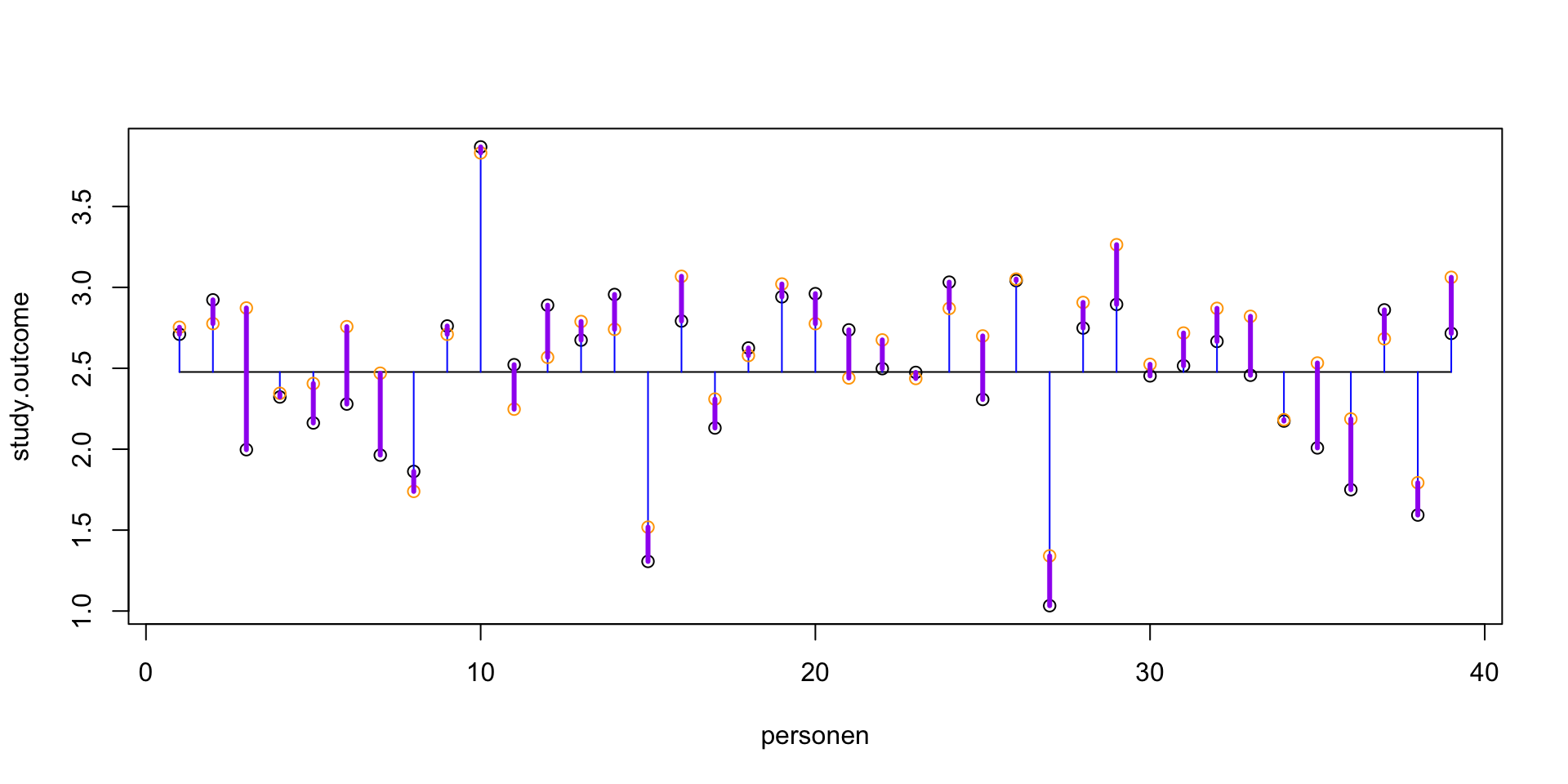
How far are we off?

error = study.outcome - model

cbind(model, study.outcome, error)[1:5,]

        model study.outcome       error
[1,] 2.753512      2.710330 -0.04318159
[2,] 2.775969      2.922617  0.14664823
[3,] 2.872561      1.997056 -0.87550534
[4,] 2.345205      2.322539 -0.02266610
[5,] 2.405860      2.162133 -0.24372667

Outcome = Model + Error

Is that true?

study.outcome == model + error

 [1] TRUE TRUE TRUE TRUE TRUE TRUE TRUE TRUE TRUE TRUE TRUE TRUE TRUE TRUE TRUE
[16] TRUE TRUE TRUE TRUE TRUE TRUE TRUE TRUE TRUE TRUE TRUE TRUE TRUE TRUE TRUE
[31] TRUE TRUE TRUE TRUE TRUE TRUE TRUE TRUE TRUE

Yes!

Visual

Explained variance

The explained variance is the deviation of the estimated model outcome compared to the total mean.

To get a percentage of explained variance, it must be compared to the total variance. In terms of squares:

\(\frac{{SS}_{model}}{{SS}_{total}}\)

We also call this: \(r^2\) of \(R^2\).

Why?

r = cor(study.outcome, model)
r^2

[1] 0.7527463

End

Contact