ANOVA

F-distribution

One-way independent ANOVA

End

Ronald Fisher

Analysing variance

Population distribution

Population distribution

F-statistic

A samples

More samples

More samples

F-distribution

F-distribution

Assumptions

Jet lag

Variance components

Total variance

Visual \({SS}_{total}\)

Visual \({SS}_{total}\)

Model variance

Visual \({SS}_{model}\)

Error variance

Visual \({SS}_{error}\)

Variance components

F-ratio

Reject \(H_0\)?

Contrasts

Contrasts

Post-hoc

Effect size \(\eta^2\)

Effect size \(\omega^2\)

Effect size \(r\)

Contact

F-distribution & One-way independent

Klinkenberg

University of Amsterdam

6 oct 2022

The F-distribution, also known as Snedecor’s F distribution or the Fisher–Snedecor distribution (after Ronald Fisher and George W. Snedecor) is, in probability theory and statistics, a continuous probability distribution. The F-distribution arises frequently as the null distribution of a test statistic, most notably in the analysis of variance; see F-test.

Wikipedia

Sir Ronald Aylmer Fisher FRS (17 February 1890 – 29 July 1962), known as R.A. Fisher, was an English statistician, evolutionary biologist, mathematician, geneticist, and eugenicist. Fisher is known as one of the three principal founders of population genetics, creating a mathematical and statistical basis for biology and uniting natural selection with Mendelian genetics.

Wikipedia

Decomposing variance example of height for males and females.

layout(matrix(c(2:6,1,1,7:8,1,1,9:13), 4, 4))

n  = 56    # Sample size
df = n - 1 # Degrees of freedom

mu    = 120
sigma = 15

IQ = seq(mu-45, mu+45, 1)

par(mar=c(4,2,0,0))  
plot(IQ, dnorm(IQ, mean = mu, sd = sigma), type='l', col="red")

n.samples = 12

for(i in 1:n.samples) {
  
  par(mar=c(2,2,0,0))  
  hist(rnorm(n, mu, sigma), main="", cex.axis=.5, col="red")
  
}

\[F = \frac{{MS}_{model}}{{MS}_{error}} = \frac{{SIGNAL}}{{NOISE}}\]

So the \(F\)-statistic represents a signal to noise ratio by deviding the model variance component by the error variance component.

Let’s take two sample from our normal populatiion and calculate the F-value.

x.1 = rnorm(n, mu, sigma)
x.2 = rnorm(n, mu, sigma)

data <- data.frame(group = rep(c("s1", "s2"), each=n), score = c(x.1,x.2))
    
F = summary(aov(lm(score ~ group, data)))[[1]]$F[1]
F

[1] 1.663476

let’s take more samples and calculate the F-value every time.

n.samples = 1000

f.values = vector()

for(i in 1:n.samples) {
  
  x.1 = rnorm(n, mu, sigma); x.1
  x.2 = rnorm(n, mu, sigma); x.2

  data <- data.frame(group = rep(c("s1", "s2"), each=n), score = c(x.1,x.2))
    
  f.values[i] = summary(aov(lm(score ~ group, data)))[[1]]$F[1]

}

k = 2
N = 2*n

df.model = k - 1
df.error = N - k

hist(f.values, freq = FALSE, main="F-values", breaks=100)
F = seq(0, 6, .01)
lines(F, df(F,df.model, df.error), col = "red")

So if the population is normaly distributed (assumption of normality) the f-distribution represents the signal to noise ration given a certain number of samples (\({df}_{model} = k - 1\)) and sample size (\({df}_{error} = N - k\)).

The F-distibution therefore is different for different sample sizes and number of groups.

Animated F-distrigutions

Compare 2 or more independent groups.

Assuming th \(H_0\) hypothesis to be true, the following should hold:

Continuous variable
Random sample
Normaly distributed
- Shapiro-Wilk test
Equal variance within groups
- Levene’s test

Wright and Czeisler (2002) performed an experiment where they measured the circadian rhythm by the daily cycle of melatonin production in 22 subjects randomly assigned to one of three light treatments.

Control condition (no light)
Knees (3 hour light to back of knees)
Eyes (3 hour light in eyes)

rm(list=ls())
x.c = c( .53, .36,  .2,  -.37, -.6,  -.64, -.68,-1.27) # Control 
x.k = c( .73, .31,  .03, -.29, -.56, -.96,-1.61      ) # Knees
x.e = c(-.78,-.86,-1.35,-1.48,-1.52,-2.04,-2.83      ) # Eyes
x   = c( x.c, x.k, x.e )                               # Conditions combined

Variance	Sum of Squares	DF	Mean Squares	F-ratio
Model	\({SS}_{model} = \sum n_k(\bar{X}_k - \bar{X})^2\)	\(k-1\)	\(\frac{{SS}_{model}}{{df}_{model}}\)	\(\frac{{MS}_{model}}{{MS}_{error}}\)
Error	\({SS}_{error} = \sum s_k^2 (n_k - 1)\)	\(N-k\)	\(\frac{{SS}_{error}}{{df}_{error}}\)
Total	\({SS}_{total} = {SS}_{model} + {SS}_{error}\)	\(N-1\)	\(\frac{{SS}_{total}}{{df}_{total}}\)

Where \(N\) is the total sample size, \(n_k\) is the sample size per category and \(k\) is the number of categories. Finally \(s_k^2\) is the variance per category.

\[{MS}_{total} = s_x^2\]

ms.t = var(x); ms.t

[1] 0.7923732

sum( (x - mean(x))^2 ) / (length(x) - 1)

[1] 0.7923732

\[{SS}_{total} = s_x^2 (N-1)\]

N = length(x)

ss.t = var(x) * (N-1); ss.t

[1] 16.63984

sum( (x - mean(x))^2 )

[1] 16.63984

# Assign labels
lab = c("Control", "Knee", "Eyes") 

# Plot all data points
plot(1:N,x, 
     ylab="Shift in circadian rhythm (h)",
     xlab="Light treatment",
     main="Total variance")

# Add mean line
lines(c(1,22),rep(mean(x),2),lwd=3)

# Add delta lines / variance components
segments(1:N, mean(x), 1:N, x)

# Add labels
text(c(4,11.5,18.5),rep(.6,3),labels=lab)

\[{MS}_{model} = \frac{{SS}_{model}}{{df}_{model}} \\ {df}_{model} = k - 1\]

Where \(k\) is the number of independent groups and

\[{SS}_{model} = \sum_{k} n_k (\bar{X}_k - \bar{X})^2\]

k      = 3
n.c = length(x.c)
n.k = length(x.k)
n.e = length(x.e)

ss.m.c = n.c * (mean(x.c) - mean(x))^2
ss.m.k = n.k * (mean(x.k) - mean(x))^2
ss.m.e = n.e * (mean(x.e) - mean(x))^2

ss.m = sum(ss.m.c, ss.m.k, ss.m.e); ss.m

[1] 7.224492

df.m = (k - 1)
ms.m = ss.m / df.m; ms.m

[1] 3.612246

\[{MS}_{error} = \frac{{SS}_{error}}{{df}_{error}} \\ {df}_{error} = N - k\]

where

\[{SS}_{error} = \sum_{k} s_k^2 (n_k - 1) = \sum_{k} \frac{\sum (x_{ik} - \bar{x}_k)^2}{(n_k - 1)} (n_k - 1)\]

ss.e.c = var(x.c) * (n.c - 1)
ss.e.k = var(x.k) * (n.k - 1)
ss.e.e = var(x.e) * (n.e - 1)
ss.e   = sum(ss.e.c, ss.e.k, ss.e.e); ss.e

[1] 9.415345

\[{MS}_{error} = \frac{{SS}_{error}}{{df}_{error}} \\ {df}_{error} = N - k\]

df.e = (N - k)
ms.e = ss.e / df.e; ms.e

[1] 0.4955445

\[{SS}_{total} = {SS}_{model} + {SS}_{error}\]

\[16.6398364 = 7.2244917 + 9.4153446\]

\[{MS}_{total} = \frac{{SS}_{total}}{{df}_{total}}= 0.7923732\]

\[{MS}_{model} = \frac{{SS}_{model}}{{df}_{model}}= 3.6122459\]

\[{MS}_{error} = \frac{{SS}_{error}}{{df}_{error}} = 0.4955445\]

\[F = \frac{{MS}_{model}}{{MS}_{error}} = \frac{{SIGNAL}}{{NOISE}}\]

F = ms.m / ms.e; F

[1] 7.289449

if(!"visualize" %in% installed.packages()) { install.packages("visualize") }
library("visualize")

visualize.f(F, df.m,df.e,section="upper")

Planned comparisons

Exploring differences of theoretical interest
Higher precision
Higher power

Only use chunks once
Values add up to 0

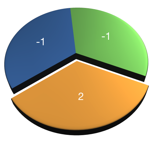
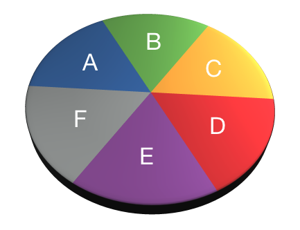
AB-CDEF → A-B → CD-EF → C-D → E-F
A-BCDEF → A-B → A-C
A-BCDEG → BC-DEF → B-C → B-DEF
ABC-DEF → BC-DEF → B-C

Assign values that combine to one. Same values define chunk.

AB-CDEF → A-B → CD-EF → C-D → E-F

Unplanned comparisons

Exploring all possible differences
Adjust T value for inflated type 1 error

	C	K	E
C		2	3
K	4		6
E	7	8

The amount of explained variance \(R^2\) as a general effect size measure.

\[R^2 = \frac{{SS}_{model}}{{SS}_{total}} = \eta^2\]

Taking the square root gives us Cohen’s \(r\).

Less biased towards just the sample is omega squared \(\omega^2\).

\[\omega^2 = \frac{{SS}_{model} - ({df}_{model}){MS}_{error}}{{SS}_{total}+{MS}_{error}}\]

But what does it say?

A more interpretable effect size measure is \(r_{Contrast}\). Which gives the effect size for a specific contrast.

\[r_{Contrast} = \sqrt{\frac{t^2}{t^2+{df}}}\]

Contrast 1

Contrast 2

Contrast 3

Contrast 4