Correlation and Simple regression
University of Amsterdam
3 nov 2022
Pearson Correlation

In statistics, the Pearson correlation coefficient, also referred to as the Pearson’s r, Pearson product-moment correlation coefficient (PPMCC) or bivariate correlation, is a measure of the linear correlation between two variables X and Y. It has a value between +1 and −1, where 1 is total positive linear correlation, 0 is no linear correlation, and −1 is total negative linear correlation. It is widely used in the sciences. It was developed by Karl Pearson from a related idea introduced by Francis Galton in the 1880s.
Source: Wikipedia
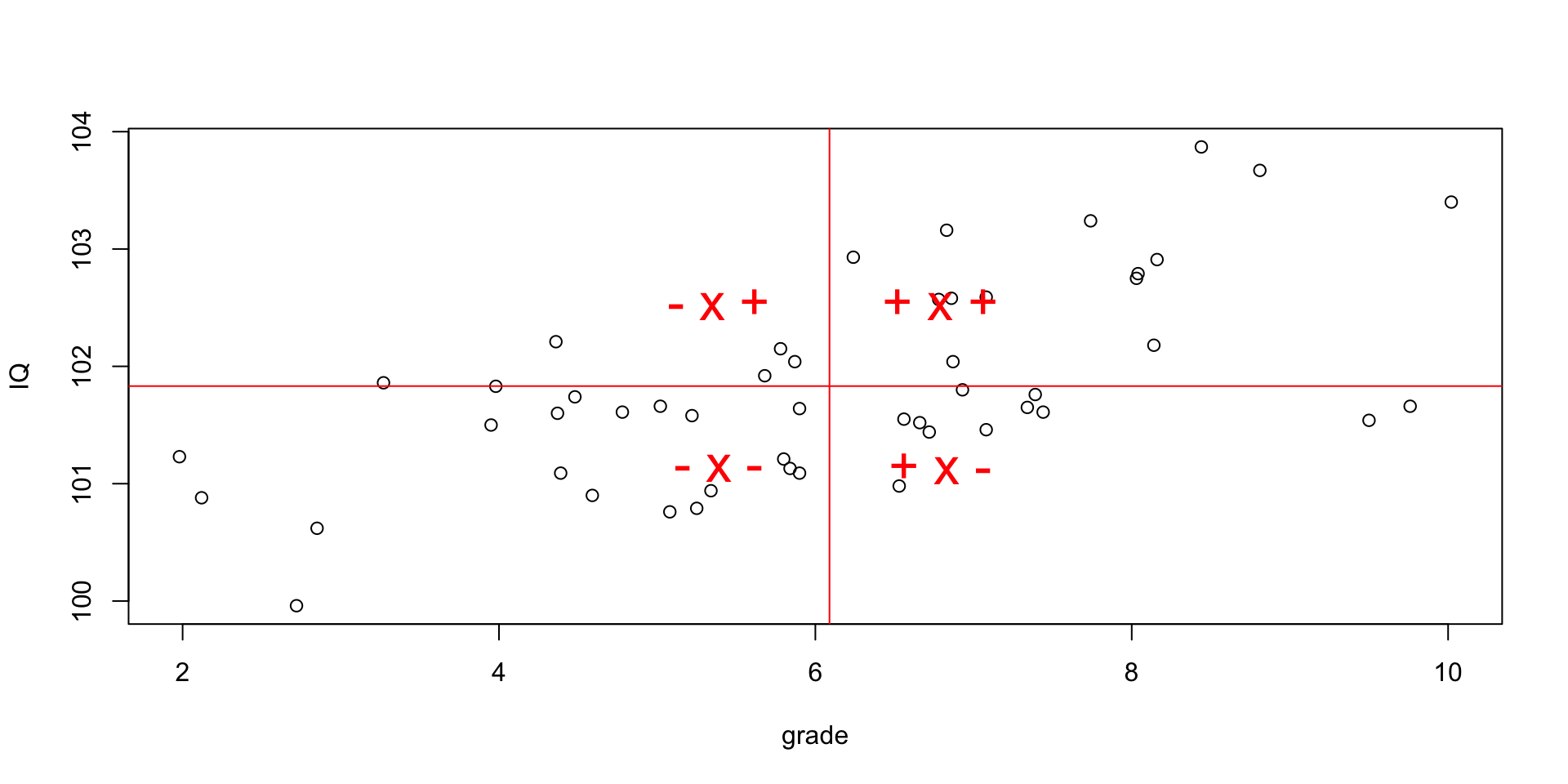
Plot correlation
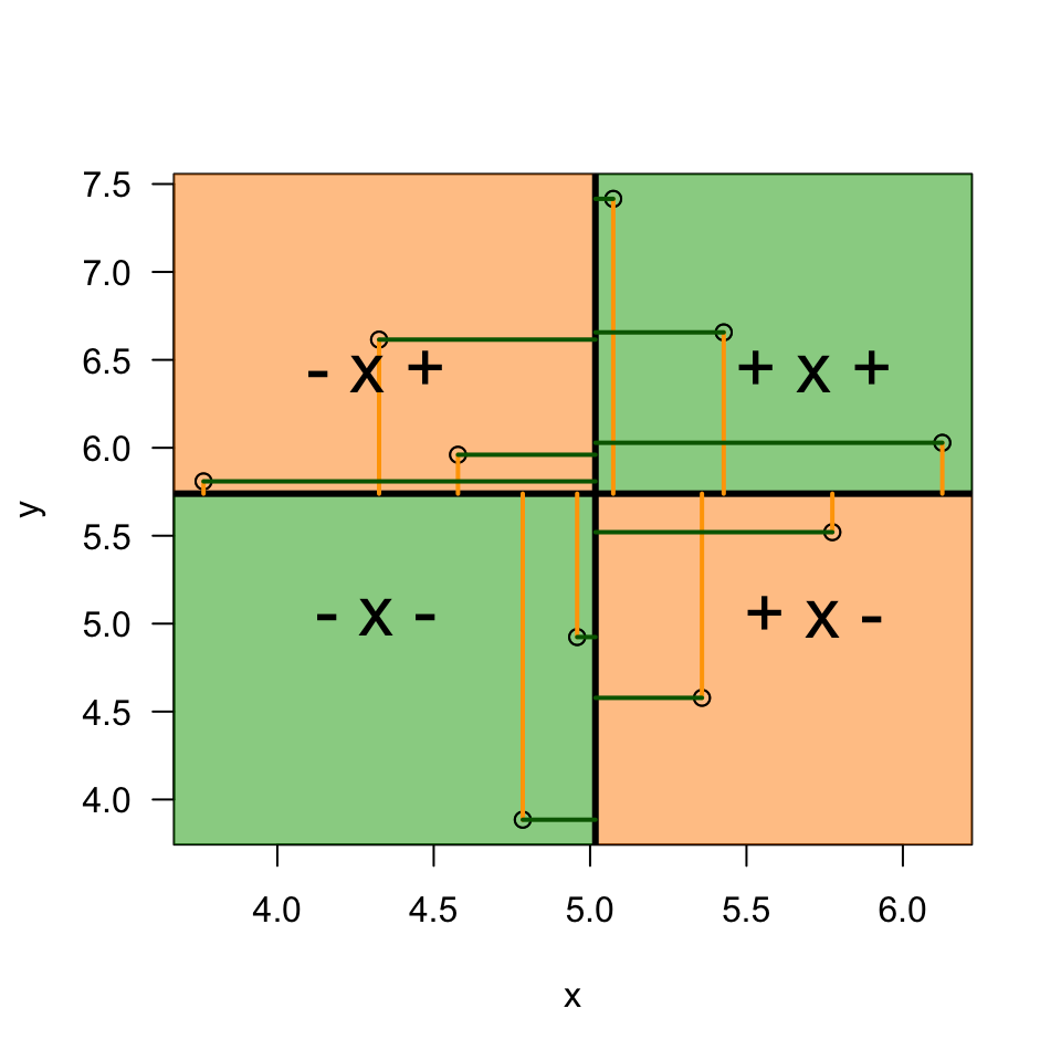
\[(x_i - \bar{x})(y_i - \bar{y})\]
Guess the correlation


Explaining vairance

Standarize

Plot correlation
Visualize

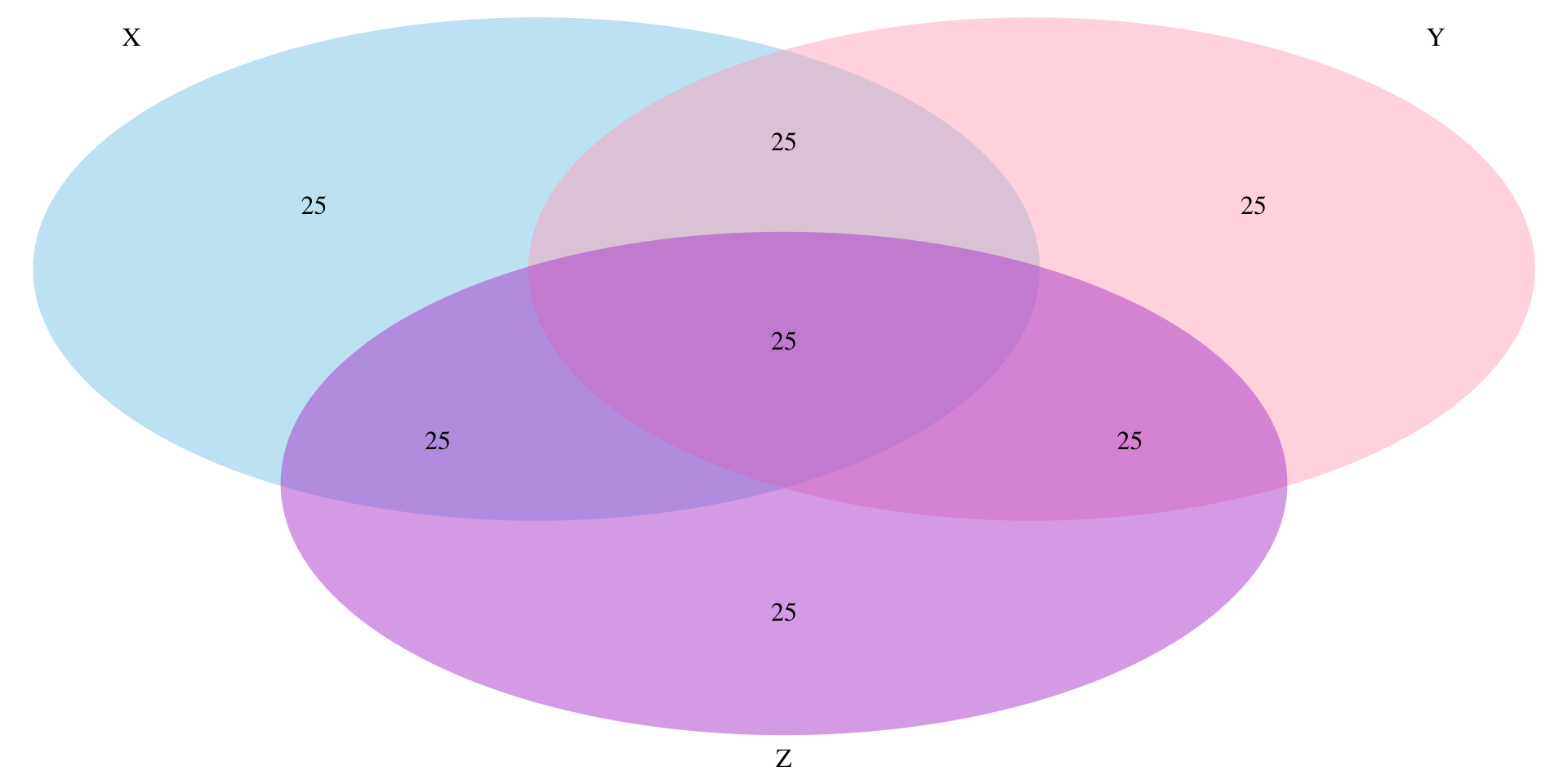
Venn diagram
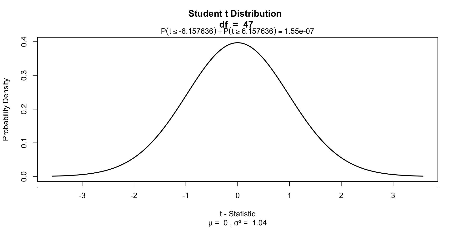
Significance of parial correlation
Outcome vs Model


Homoscedasticity
- Variance of residual should be equal across all expected values
- Look at scatterplot of standardized: expected values \(\times\) residuals. Roughly round shape is needed.

The slope


P-values of \(b_0\)
P-values of \(b_1\)

\(y\) vs \(\hat{y}\)
And lets have a look at this relation between expectation and reality

Explained variance visually

The part that does not overlap is therefore ‘unexplained’ variance. And because \(r^2\) is the explained variance, \(1 - r^2\) is the unexplained variance.
Visualize

Contact

![]()