ANOVA

Repeated & Mixed

ANOVA
One-way repeated

One-way repeated measures ANOVA

The one-way repeated measures ANOVA analyses the variance of the model while reducing the error by the within person variance.

• 1 dependent/outcome variable
• 1 independent/predictor variable
  • 2 or more levels
• All with same subjects

Assumptions

• Uni- or Multivariate
• Continuous dependent variable
• Normaly distributed
  • Shapiro-Wilk
• Equality of variance within groups
  • Mauchly’s test of Sphericity

Uni- or Multi- descision tree

Decision tree

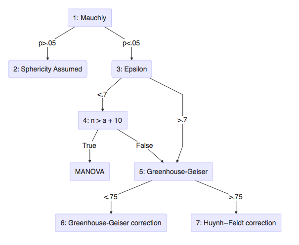
1. Field: 15.5.2, Output 15.2
2. Field: Output 15.4
3. Field: Jane Superbrain 15.2, Output 15.2 GG and HF.
4. Field: Jane Superbrain 15.2, Sample size \(n\) is larger than \(a\) (number of levels) + 10
5. Field: 15.5.4, Output 15.2
6. Field: 15.5.4, Output 15.4
7. Field: 15.5.4, Output 15.4

Formulas

Variance	Sum of Squares	df	Mean Squares	F-ratio
Between	\({SS}_{{between}} = {SS}_{{total}} - {SS}_{{within}}\)	\({DF}_{{total}}-{DF}_{{within}}\)	\(\frac{{SS}_{{between}}}{{DF}_{{between}}}\)
Within	\({SS}_{{within}} = \sum{s_i^2(n_i-1)}\)	\((n_i-1)n\)	\(\frac{{SS}_{{within}}}{{DF}_{{within}}}\)
• Model	\({SS}_{{model}} = \sum{n_k(\bar{X}_k-\bar{X})^2}\)	\(k-1\)	\(\frac{{SS}_{{model}}}{{DF}_{{model}}}\)	\(\frac{{MS}_{{model}}}{{MS}_{{error}}}\)
• Error	\({SS}_{{error}} = {SS}_{{within}} - {SS}_{{model}}\)	\((n-1)(k-1)\)	\(\frac{{SS}_{{error}}}{{DF}_{{error}}}\)
Total	\({SS}_{{total}} = s_{grand}^2(N-1)\)	\(N-1\)	\(\frac{{SS}_{{total}}}{{DF}_{{total}}}\)

Where \(n_i\) is the number of observations per person and \(k\) is the number of conditions. These two are equal for a one-way repeated ANOVA. Furthermore \(n\) is the number of subjects per condition and \(N\) is the total number of data points \(n \times k\).

Example

Measure driving ability in a driving simulator. Test in three consecutive conditions where participants come back to attend the next condition.

• Alcohol none
• Alcohol some
• Alcohol much

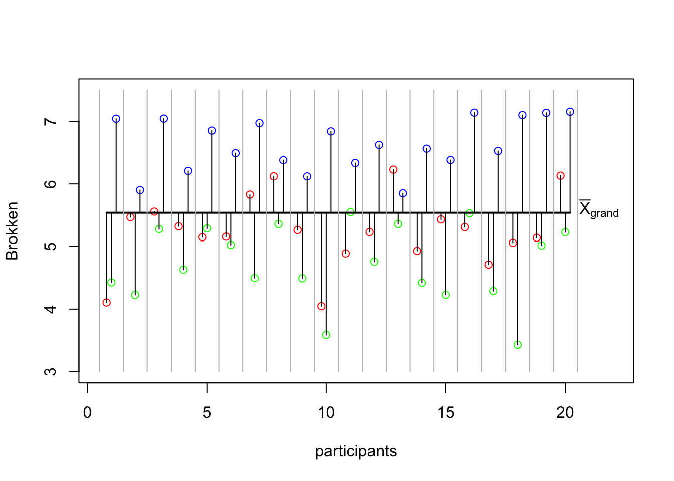
The data

MS total

# Assign to individual variables
none_alc = data$none_alc
some_alc = data$some_alc
much_alc = data$much_alc
total    = c(none_alc,some_alc,much_alc)

\({MS}_{total} = \frac{{SS}_{{total}}}{{DF}_{{total}}} = s_{grand}^2\)

MS_total = var(total); MS_total

[1] 0.9410458

SS total

\({DF_{total}} = N-1\)

\({SS}_{{total}} = s_{grand}^2(N-1)\)

N = length(total)
DF_total = N - 1
SS_total = MS_total * DF_total; SS_total

[1] 55.5217

sum((total - mean(total))^2)

[1] 55.5217

SS total visual

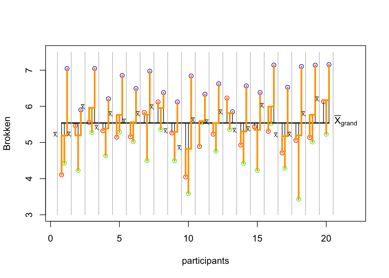
MS within

\({MS}_{within} = \frac{{SS}_{{within}}}{{DF}_{{within}}} \\ {DF}_{within} = (n_i-1)n\)

n.i = 3  # Number of mesurements per individual (none, some, much)
n   = 20 # Number of mesurements per group

DF_within = (n.i - 1) * n
DF_within

[1] 40

SS within

\({SS}_{{within}} = \sum{s_i^2(n_i-1)}\)

var_pp = apply(cbind(none_alc, some_alc, much_alc),1,var)
ss_pp  = var_pp * (n.i - 1)

SS_within = sum(ss_pp); SS_within

[1] 48.45032

mean_pp = apply(cbind(none_alc, some_alc, much_alc),1,mean)

sum(c((none_alc - mean_pp)^2, 
      (some_alc - mean_pp)^2,
      (much_alc - mean_pp)^2))

[1] 48.45032

SS within data

SS within visual

MS between

\({MS}_{between} = \frac{{SS}_{{between}}}{{DF}_{{between}}}\)

\({DF}_{between}-{DF}_{{within}} \\ {SS}_{between} = {SS}_{total} - {SS}_{within}\)

SS_between = SS_total - SS_within
SS_between

[1] 7.071382

DF_between = DF_total - DF_within
DF_between

[1] 19

MS model

\({MS}_{model} = \frac{{SS}_{{model}}}{{DF}_{{model}}} \\ {DF}_{model} = k-1\)

k = 3
DF_model = k - 1
DF_model

[1] 2

SS model

\({SS}_{model} = \sum{n_k(\bar{X}_k-\bar{X})^2}\)

# SS model
n_k1 = length(none_alc)
n_k2 = length(some_alc)
n_k3 = length(much_alc)

# Calculate sums of squares for the model
SS_k1 = n_k1 * (mean(none_alc) - mean(total))^2
SS_k2 = n_k2 * (mean(some_alc) - mean(total))^2
SS_k3 = n_k3 * (mean(much_alc) - mean(total))^2

SS_model = sum(SS_k1, SS_k2, SS_k3)
SS_model

[1] 38.63266

SS model visual

p
# Add the no alcohol mean
lines(c((1),(n)),rep(mean(none_alc),2),col='green',lwd=2)
text(n+offset,mean(none_alc),expression(bar(X)[none]),pos=4)

# With the bit alcohol mean
lines(c((1-offset),(n-offset)),rep(mean(some_alc),2),col='red',lwd=2)
text(n+offset,mean(some_alc),expression(bar(X)[some]),pos=4)

# With the much alcohol mean
lines(c((1+offset),(n+offset)),rep(mean(much_alc),2),col='blue',lwd=2)
text(n+offset,mean(much_alc),expression(bar(X)[much]),pos=4)

# The lines show the model deviation from the total mean.
segments(1:n,        mean(total), 1:n,        mean(none_alc),   col='green')
segments(1:n-offset, mean(total), 1:n-offset, mean(some_alc), col='red')
segments(1:n+offset, mean(total), 1:n+offset, mean(much_alc),   col='blue')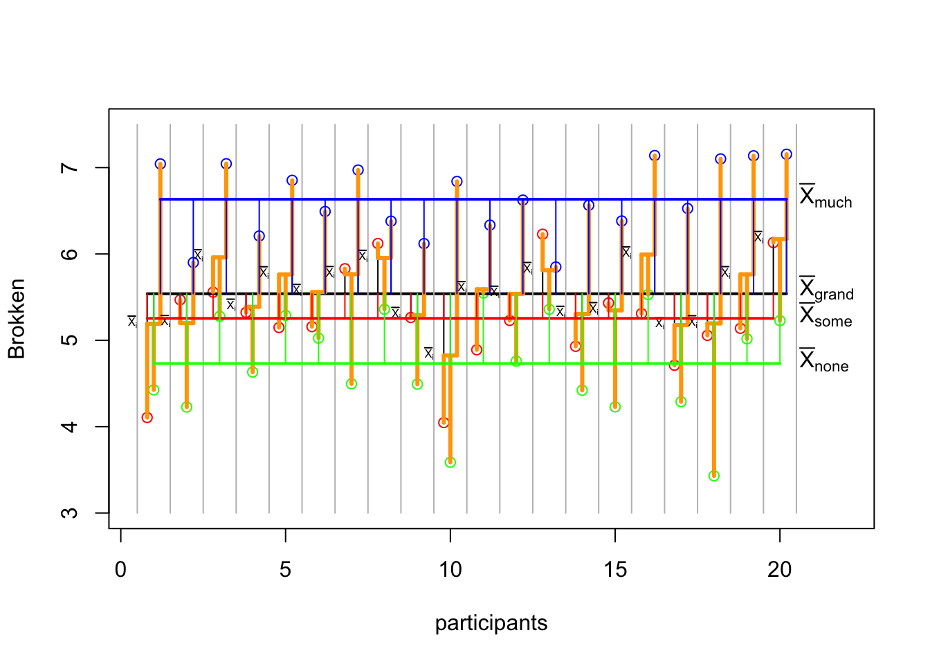

p <- recordPlot()

MS error

\(\frac{{SS}_{error}}{{DF}_{error}}\)

\({DF}_{error} = (n-1)(k-1)\)

DF_error = DF_within - DF_model
DF_error

[1] 38

SS error

\({SS}_{error} = {SS}_{within} - {SS}_{model}\)

SS_error = SS_within - SS_model
SS_error

[1] 9.817655

F ratio

\(F = \frac{{MS}_{{model}}}{{MS}_{{error}}}\)

# Calculate mean squares
MS_model = SS_model / DF_model
MS_error = SS_error / DF_error

# Calculate F statistic
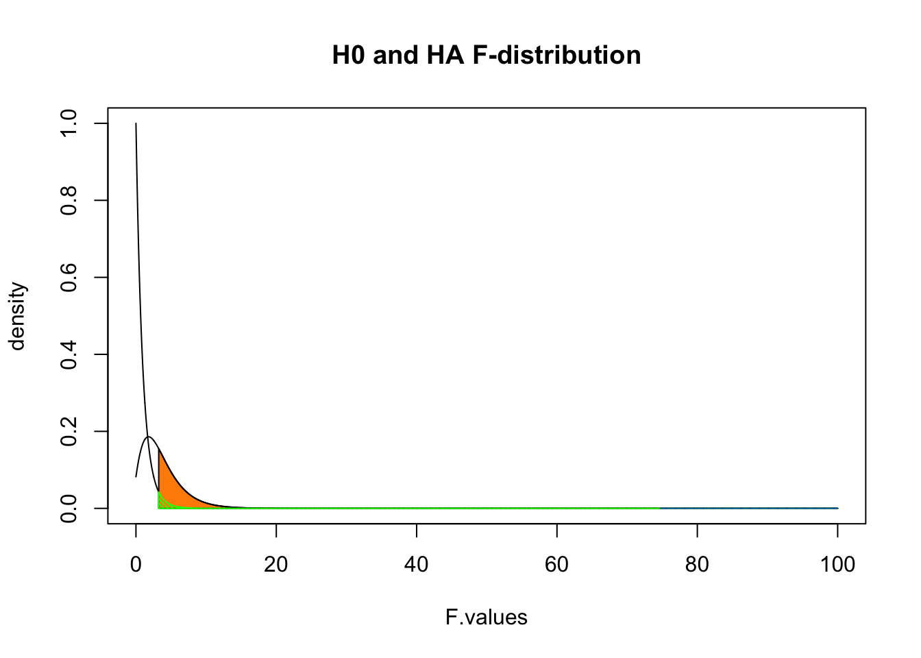
F = MS_model / MS_error
F

[1] 74.76537

Visualize

library('visualize')
visualize.f(F, DF_model, DF_error, section="upper")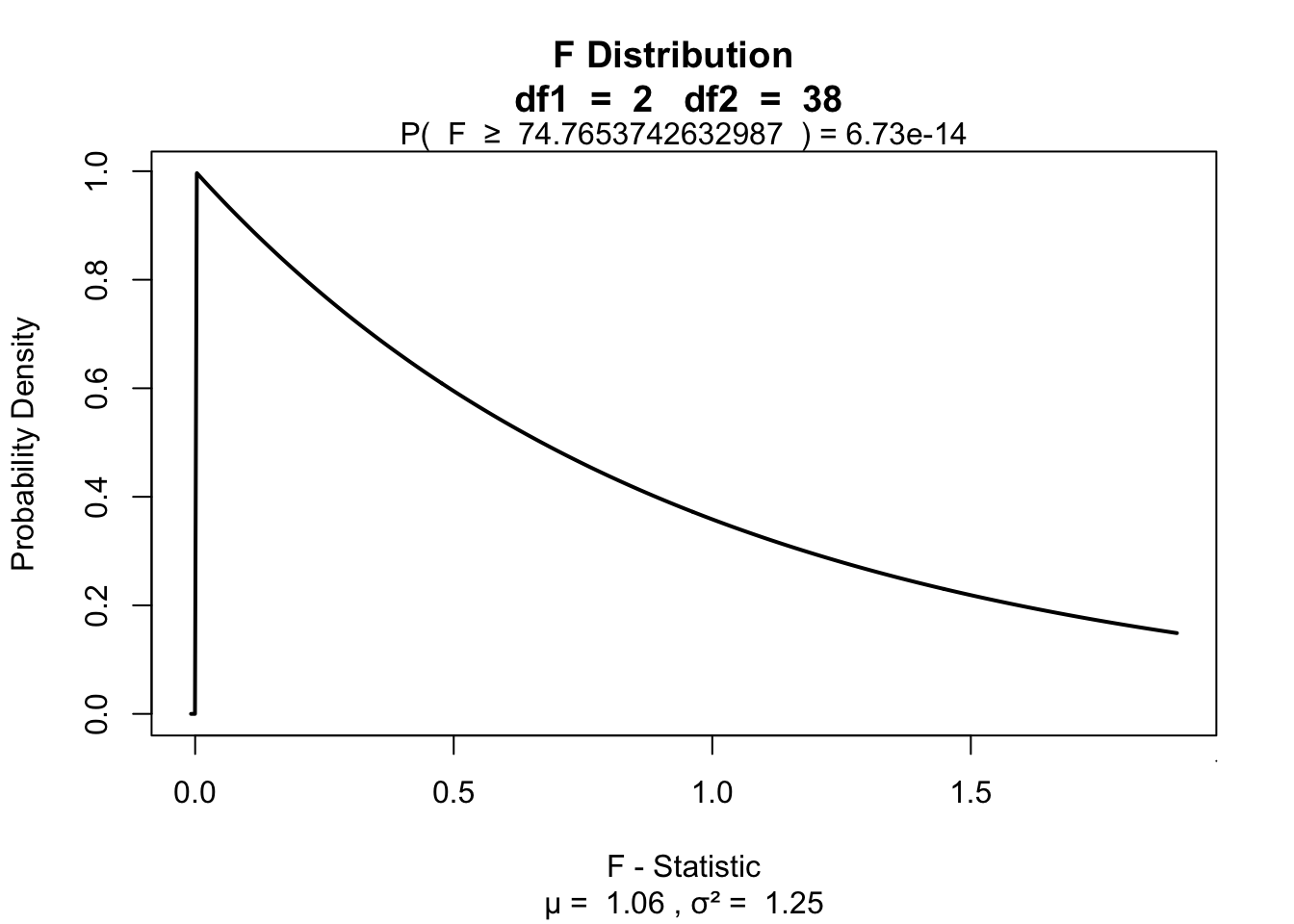

Contrast

Planned comparisons

• Exploring differences of theoretical interest
• Higher precision
• Higher power

Post-Hoc

Unplanned comparisons

• Exploring all possible differences
• Adjust T value for inflated type 1 error

Effect size

General effect size measures

• Amount of explained variance \(R^2\) also called eta squared \(\eta^2\).
• Omega squared \(\omega^2\)

Effect sizes of contrasts or post-hoc comparisons

• Cohen’s \(r\) gives the effect size for a specific comparison
  • \(r_{Contrast} = \sqrt{\frac{t^2}{t^2+{df}}}\)
  • \(r_{Contrast} = \sqrt{\frac{F(1,{df}_R)}{F(1,{df}_R)+{df}_R}}\)

ANOVA factorial repeated

Factorial repeated measures ANOVA

The factorial repeated measures ANOVA analyses the variance of the model while reducing the error by the within person variance.

• 1 dependent/outcome variable
• 2 or more independent/predictor variable
  • 2 or more levels
• All with same subjects

Assumptions

Same as one-way repeated measures ANOVA

Example

In this example we will again look at the amount of accidents in a car driving simulator while subjects where given varying doses of speed and alcohol. But this time we lat participants partake in all conditions. Every week subjects returned for a different experimental condition.

• Dependent variable
  • Accidents
• Independent variables
  • Speed
    • None
    • Small
    • Large
  • Alcohol
    • None
    • Small
    • Large

person	1_1	1_2	1_3	2_1	2_2	2_3	3_1	3_2	3_3
1	1
2		2
3			3
4				4
5					5
6						6
7							7
8								8
9									9

Data

Mixed design ANOVA

Mixed design

The mixed ANOVA analyses the variance of the model while reducing the error by the within person variance.

• 1 dependent/outcome variable
• 2 or more independent/predictor variable with different subjects
  • 2 or more levels
• 1 or more independent/predictor variable with same subjects
  • 2 or more levels

Assumptions

Same as repeated measures ANOVA and same as factorial ANOVA.

Example

• Dependent variable
  • Accidents
• Independent variables
  • Speed (same subjects)
    • None
    • Small
    • Large
  • Alcohol (same subjects)
    • None
    • Small
    • Large
  • Gender
    • Males
    • Females

person	gender	1_1	1_2	1_3	2_1	2_2	2_3	3_1	3_2	3_3
1	males	1
2	males		2
3	males			3
4	males				4
5	males					5
6	males						6
7	males							7
8	males								8
9	males									9
10	females	1
12	females		2
13	females			3
14	females				4
15	females					5
16	females						6
17	females							7
18	females								8
20	females									9

Data

End

Contact

• @shklinkenberg
• Klinkenberg
• ln.AvU@grebneknilK.S
• ShKlinkenberg

CC BY-NC-SA 4.0