ANCOVA

Author

Klinkenberg

Published

October 12, 2022

ANCOVA

Analysis of covariance (ANCOVA) is a general linear model which blends ANOVA and regression. ANCOVA evaluates whether population means of a dependent variable (DV) are equal across levels of a categorical independent variable (IV) often called a treatment, while statistically controlling for the effects of other continuous variables that are not of primary interest, known as covariates (CV).

WIKIPEDIA

ANCOVA

Determine main effect while correcting for covariate

1 dependent variable
1 or more independent variables
1 or more covariates

A covariate is a variable can be a confounding variable biasing your results. By adding a covariate we reduce error/residual in the model.

Assumptions

Same as ANOVA
Independence of the covariate and treatment effect §12.3.1.
- No difference on ANOVA with covar and independent variable
- Matching experimental groups on the covariate
Homogeneity of regression slopes §12.3.2.
- Visual: scatterplot dep var * covar per condition
- Testing: interaction indep. var * covar

Data example

We want to test the difference in national extraversion but want to controll for openness to experience.

Dependent variable: Extraversion
Independent variabele: Nationality
- Dutch
- German
- Belgian
Covariate: Openness to experience

Simulate data

# Simulate data
n = 20
k = 3
group       = round(runif(n,1,k),0)
mu.covar    = 8
sigma.covar = 1
covar       = round(rnorm(n,mu.covar,sigma.covar),2)

# Create dummy variables
dummy.1 <- ifelse(group == 2, 1, 0)
dummy.2 <- ifelse(group == 3, 1, 0)

# Set parameters
b.0 = 15 # initial value for group 1
b.1 = 3  # difference between group 1 and 2
b.2 = 4  # difference between group 1 and 3
b.3 = 3  # Weight for covariate

# Create error
error = rnorm(n,0,1)

Define the model

\({outcome} = {model} + {error}\) \({model} = {indvar} + {covariate} = {nationality} + {openness}\)

Formal model

\(b_0 + b_1 {dummy}_1 + b_2 {dummy}_2 + b_3 covar\)

# Define model
outcome = b.0 + b.1 * dummy.1 + b.2 * dummy.2 + b.3 * covar + error

Dummies

The data

Group means

aggregate(outcome ~ group, data, mean)

  group  outcome
1     1 38.67000
2     2 42.16625
3     3 43.79800

Model fit no covar

What are the beta coëfficients based on the data without the covariate?

fit.group <- lm(outcome ~ factor(group), data); fit.group


Call:
lm(formula = outcome ~ factor(group), data = data)

Coefficients:
   (Intercept)  factor(group)2  factor(group)3  
        38.670           3.496           5.128

fit.group$coefficients[2:3] + fit.group$coefficients[1]

factor(group)2 factor(group)3 
      42.16625       43.79800

\({Dutch} = 38.67 \> {German} = 42.16625 \> {Belgian} = 43.798\)

Model fit only covar

What is the weight of only the covariate?

fit.covar <- lm(outcome ~ covar, data)
fit.covar


Call:
lm(formula = outcome ~ covar, data = data)

Coefficients:
(Intercept)        covar  
     15.667        3.185

Model fit with covar

fit <- lm(outcome ~ factor(group) + covar, data); fit


Call:
lm(formula = outcome ~ factor(group) + covar, data = data)

Coefficients:
   (Intercept)  factor(group)2  factor(group)3           covar  
        15.965           2.769           4.181           2.881

fit$coefficients[2:3] + fit$coefficients[1]

factor(group)2 factor(group)3 
      18.73401       20.14609

\({Dutch} = 15.96 \> {German} = 18.73 \> {Belgian} = 20.14\)

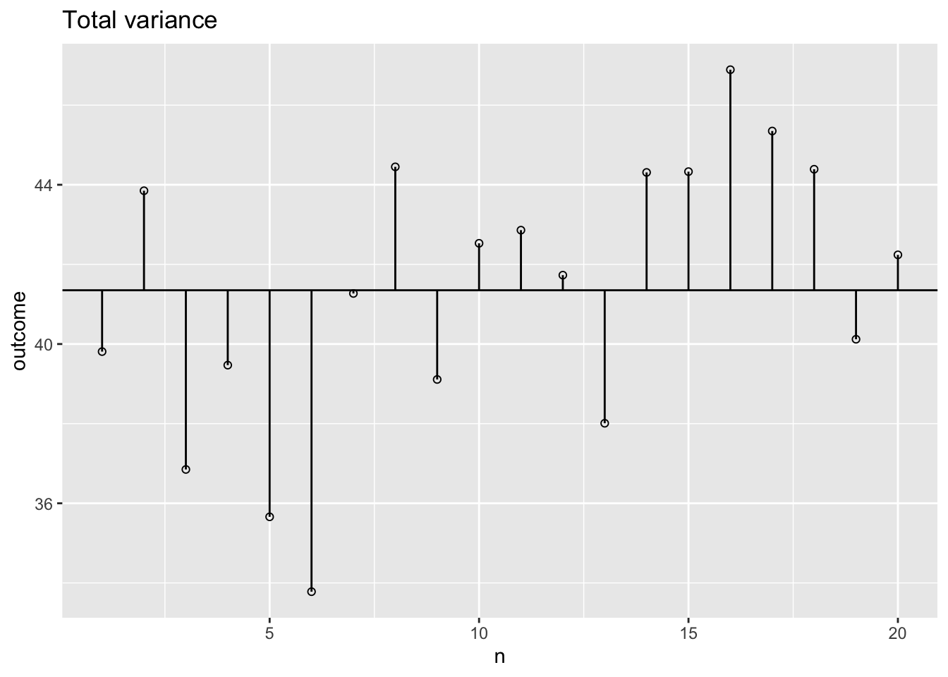
Total variance

What is the total variance

\({MS}_{total} = s^2_{outcome} = \frac{{SS}_{outcome}}{{df}_{outcome}}\)

ms.t = var(data$outcome); ms.t

[1] 11.97756

ss.t = var(data$outcome) * (length(data$outcome) - 1); ss.t

[1] 227.5737

The data

Total variance visual

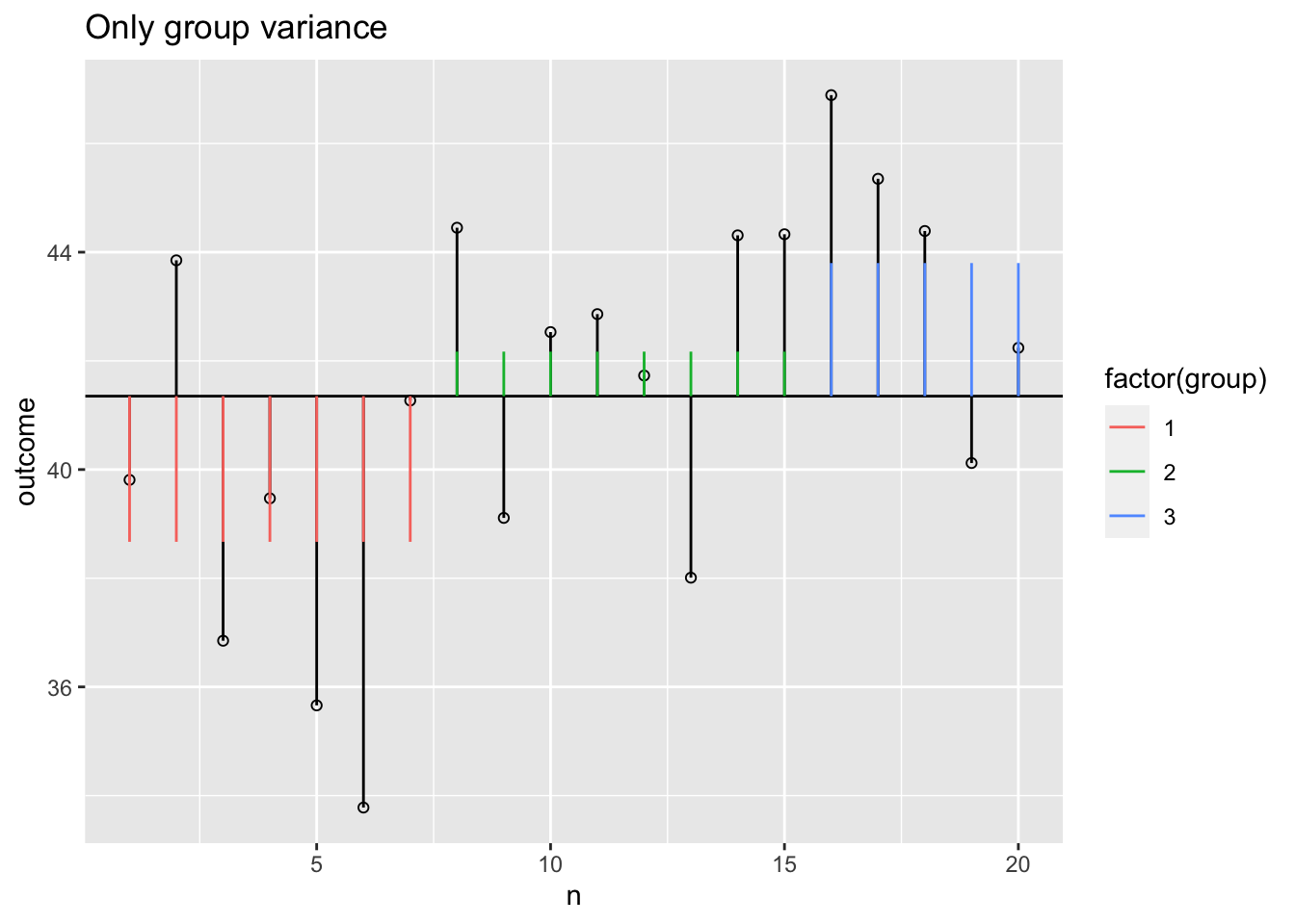
Model variance group

The model variance consists of two parts. One for the independent variable and one for the covariate. Lets first look at the independent variable.

Model variance group visual

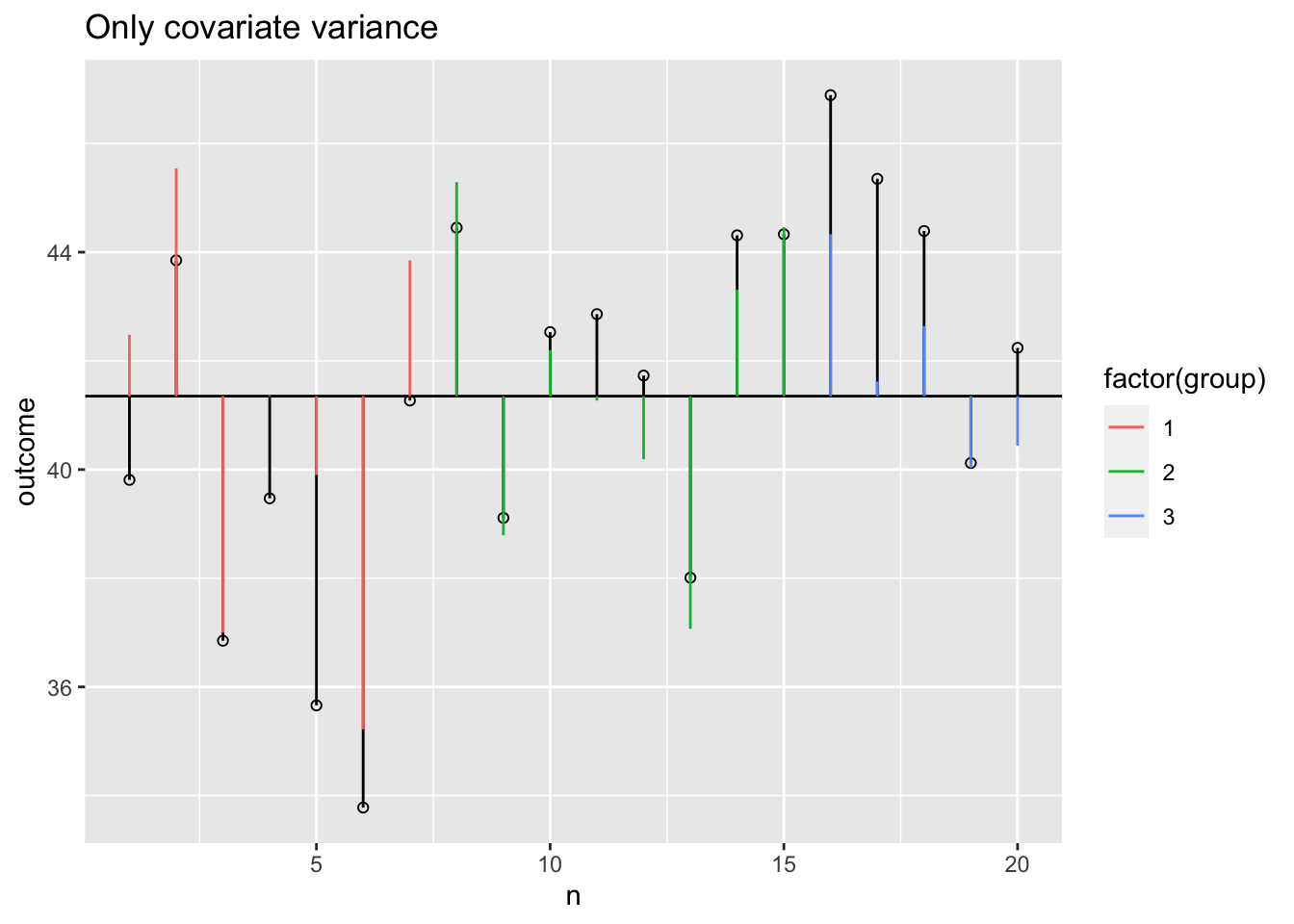
Model variance covariate visual

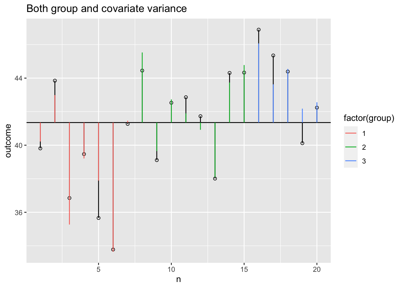
Model variance group and covariate

Model variance group and covariate visual

Error variance with covariate

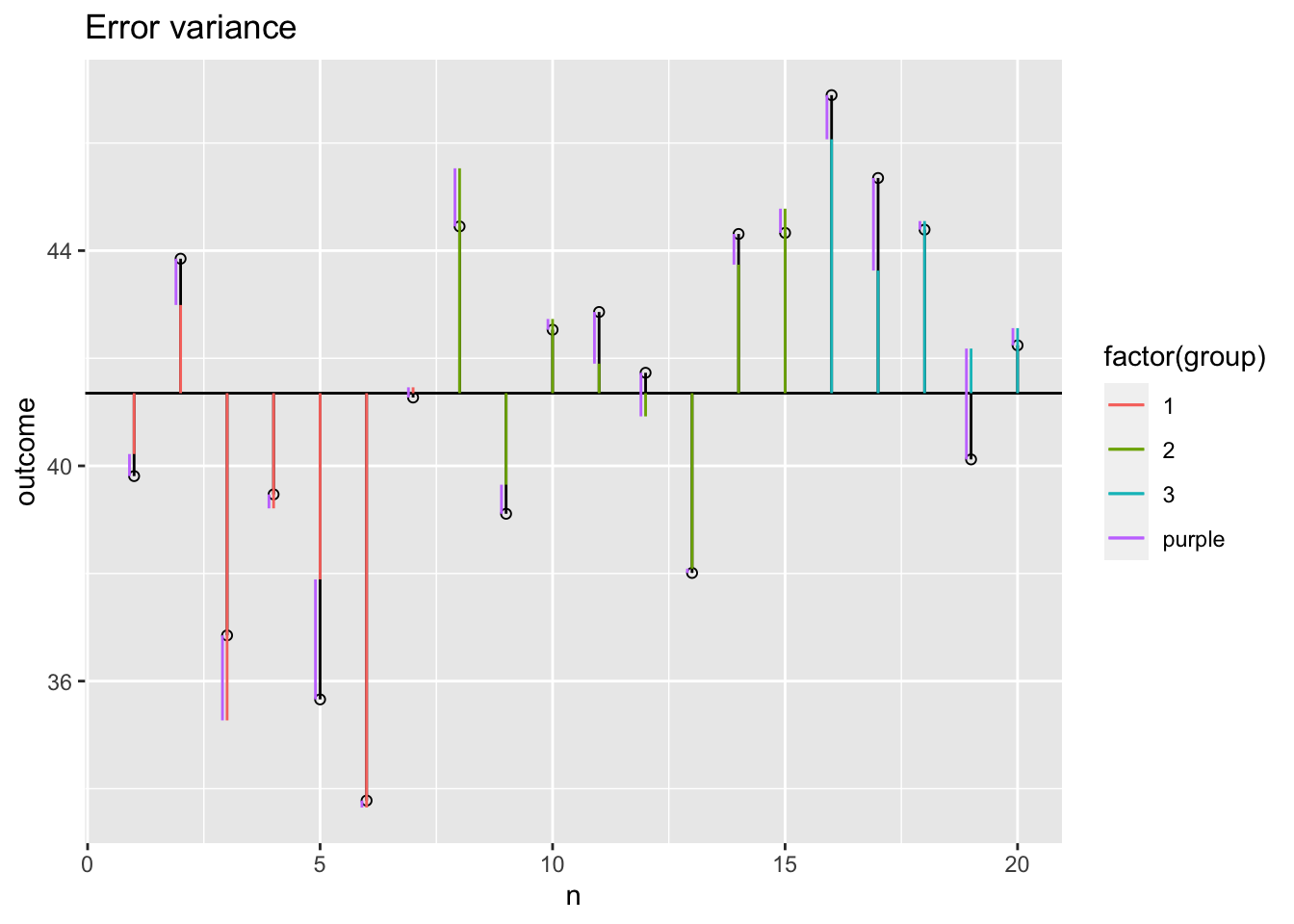
Sums of squares

SS.model = with(data, sum((model - grand.mean)^2))
SS.error = with(data, sum((outcome - model)^2))

# Sums of squares for individual effects
SS.model.group = with(data, sum((model.group - grand.mean)^2))
SS.model.covar = with(data, sum((model.covar - grand.mean)^2))

SS.covar = SS.model - SS.model.group; SS.covar ## SS.covar corrected for group

[1] 121.8463

SS.group = SS.model - SS.model.covar; SS.group ## SS.group corrected for covar

[1] 54.65778

F-ratio

\(F = \frac{{MS}_{model}}{{MS}_{error}} = \frac{{SIGNAL}}{{NOISE}}\)

n = 20
k = 3
df.model = k - 1
df.error = n - k - 1

MS.model = SS.group / df.model
MS.error = SS.error / df.error
  
F = MS.model / MS.error
F

[1] 21.74406

\(P\)-value

library("visualize")
visualize.f(F, df.model, df.error, section = "upper")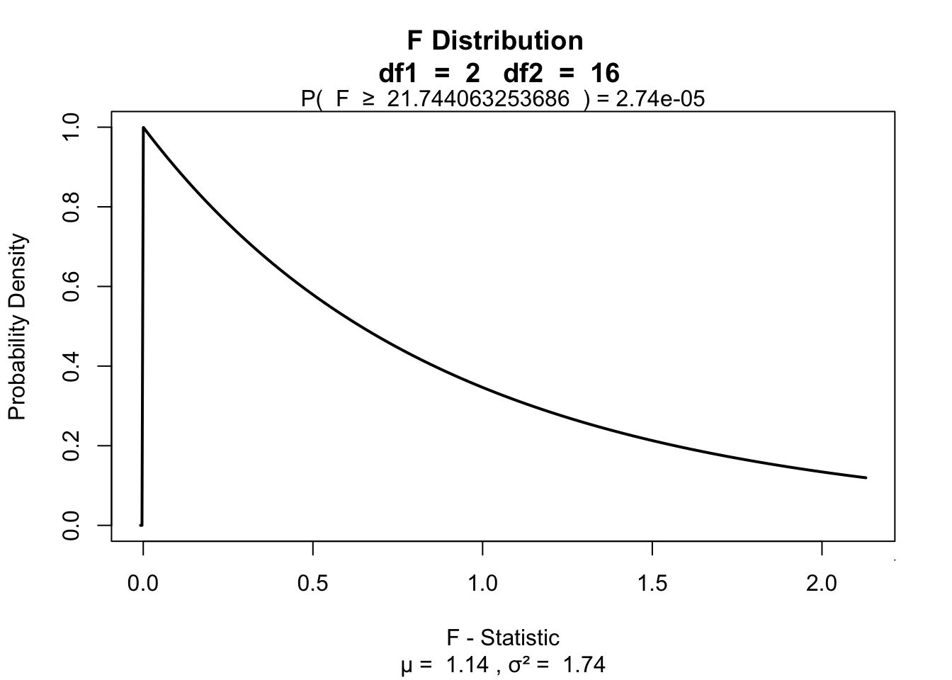

Alpha & Power

Adjusted means

# Add dummy variables
data$dummy.1 <- ifelse(data$group == 2, 1, 0)
data$dummy.2 <- ifelse(data$group == 3, 1, 0)

# b coefficients
b.cov = fit$coefficients["covar"];          b.int = fit$coefficients["(Intercept)"]
b.2   = fit$coefficients["factor(group)2"]; b.3   = fit$coefficients["factor(group)3"]

# Adjustment factor for the means of the independent variable
data$mean.adj <- with(data, b.int + b.cov * mean(covar) + b.2 * dummy.1 + b.3 * dummy.2)

aggregate(mean.adj ~ group, data, mean)

  group mean.adj
1     1 39.18576
2     2 41.95576
3     3 43.36576

Real \(\beta\)’s

b.0 = 15 # initial value for group 1
b.1 = 3  # difference between group 1 and 2
b.2 = 4  # difference between group 1 and 3
b.3 = 3  # Weight for covariate

cbind(m.covar = mu.covar*3, 
      BETA    = c(b.0, b.0+b.1, b.0+b.2), 
      sum     = mu.covar*3 + c(b.0, b.0+b.1, b.0+b.2))

     m.covar BETA sum
[1,]      24   15  39
[2,]      24   18  42
[3,]      24   19  43

End

Contact