In statistics, linear regression is a linear approach for modeling the relationship between a scalar dependent variable y and one or more explanatory variables denoted as X.
In linear regression, the relationships are modeled using linear predictor functions whose unknown model parameters \(\beta\)’s are estimated from the data (\(b\)).
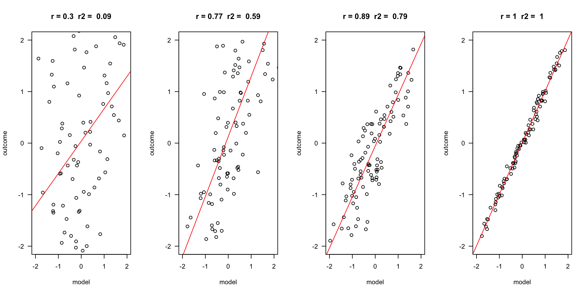
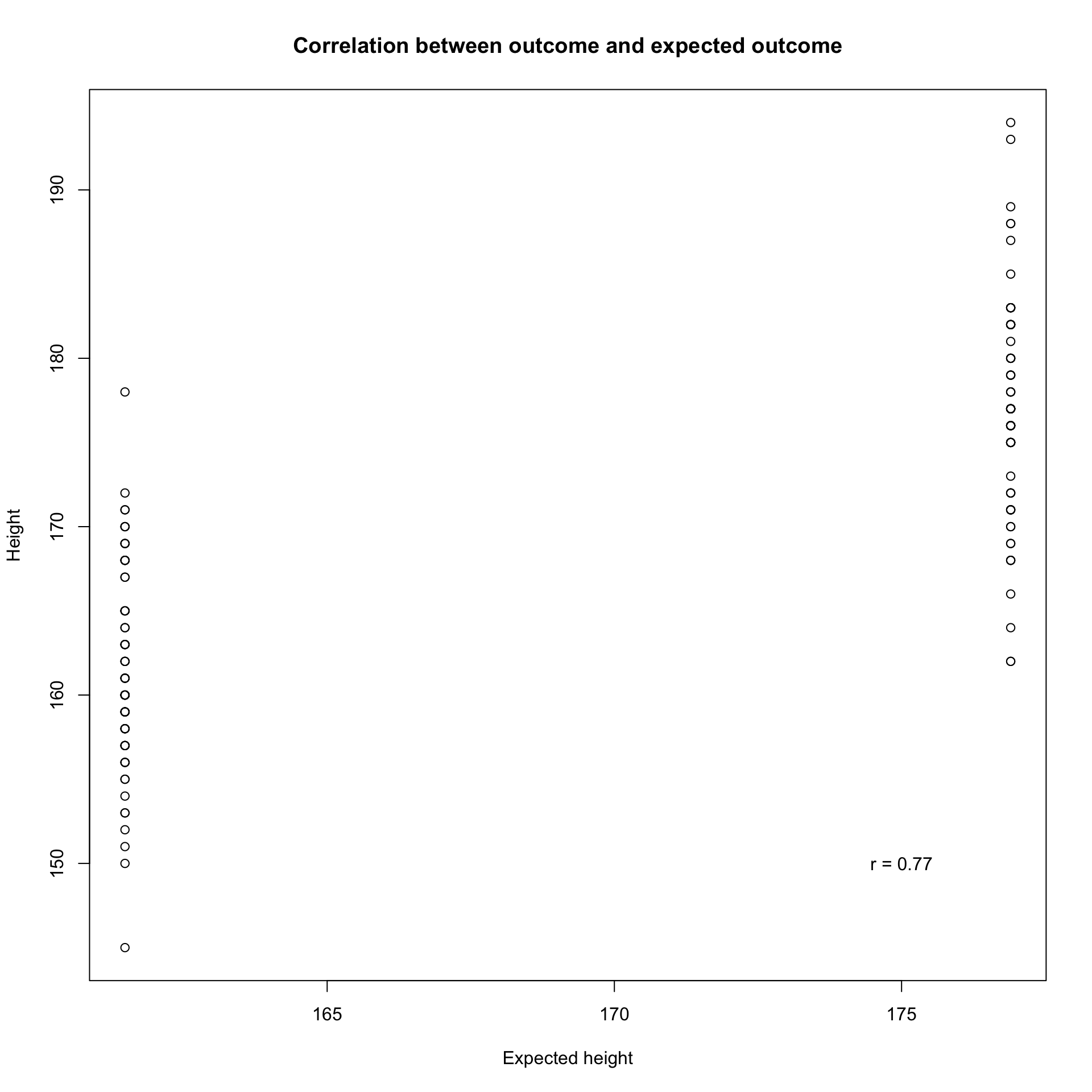
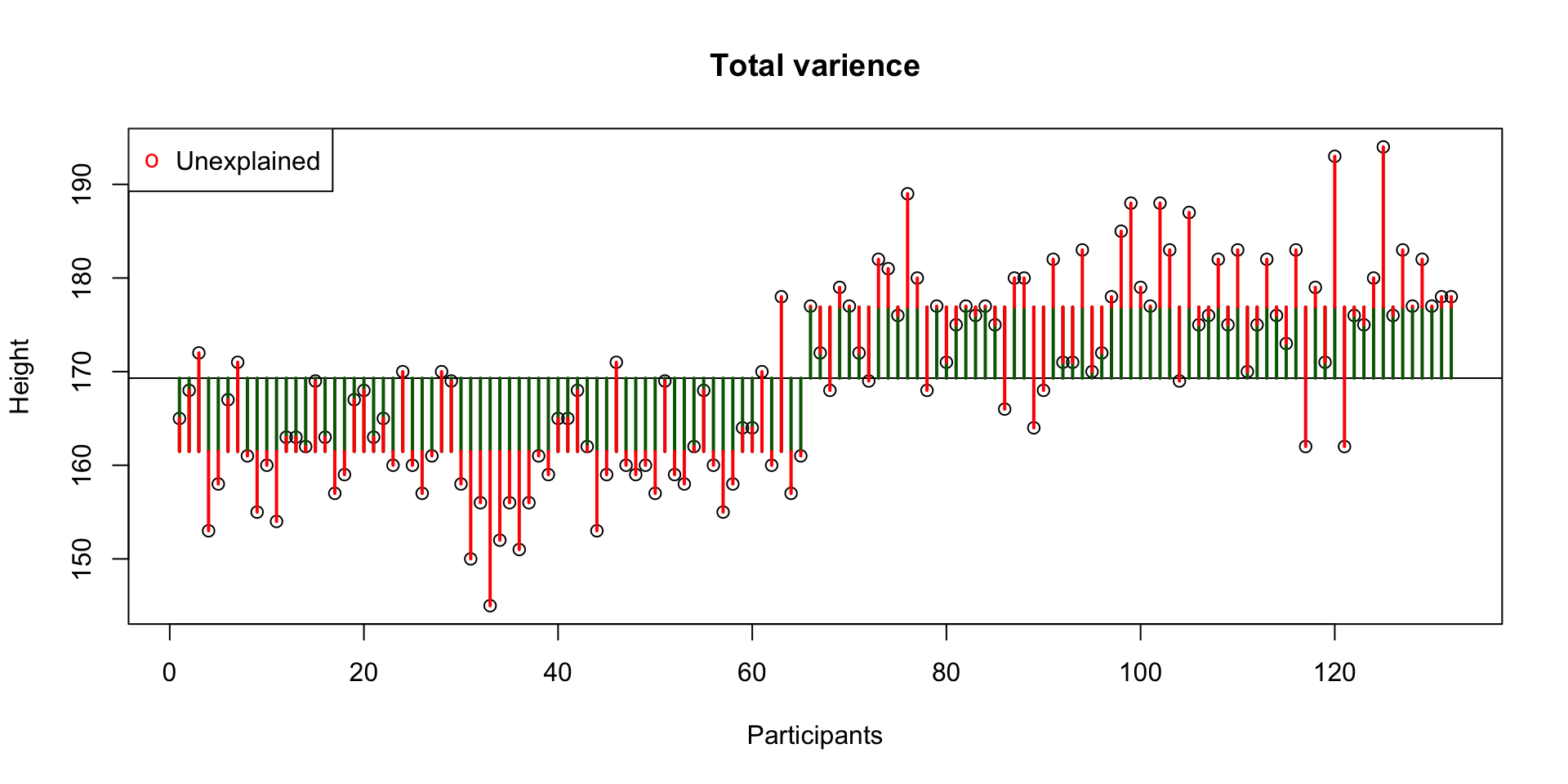
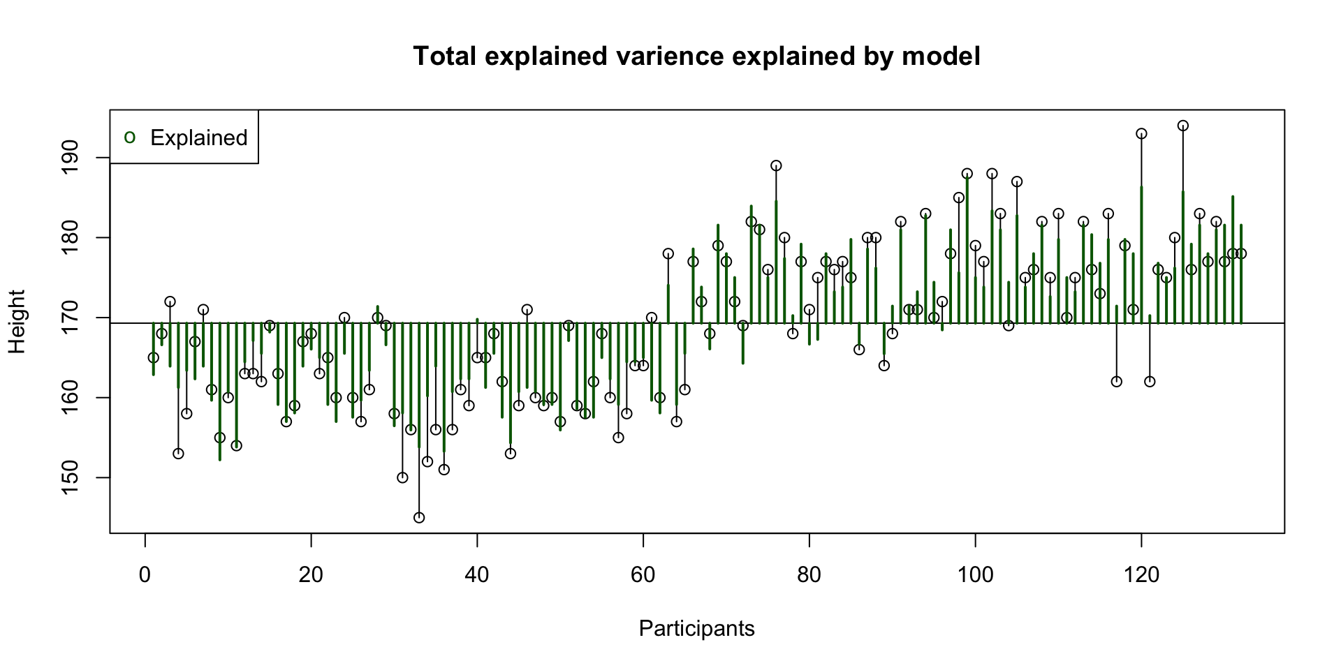
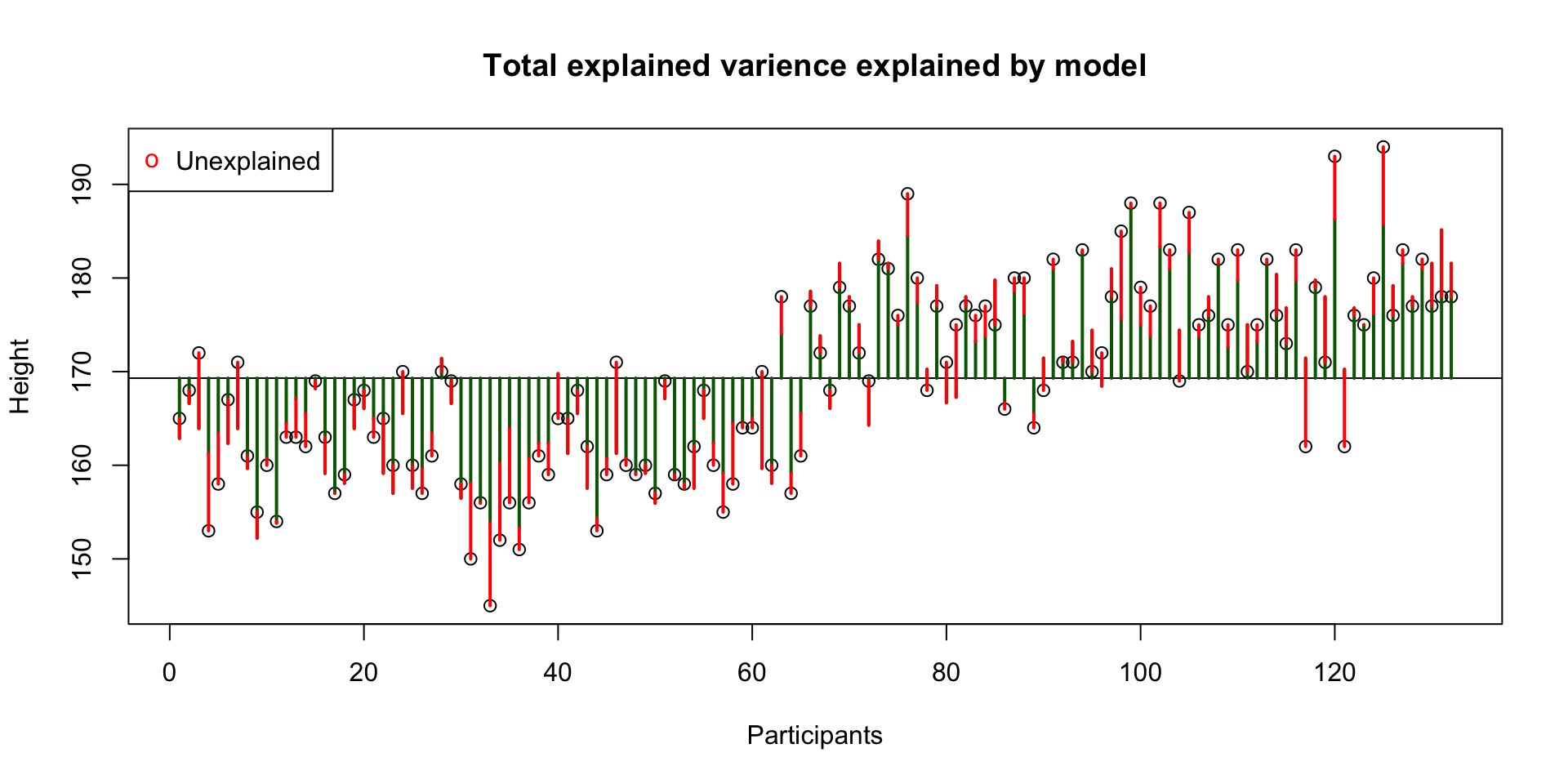
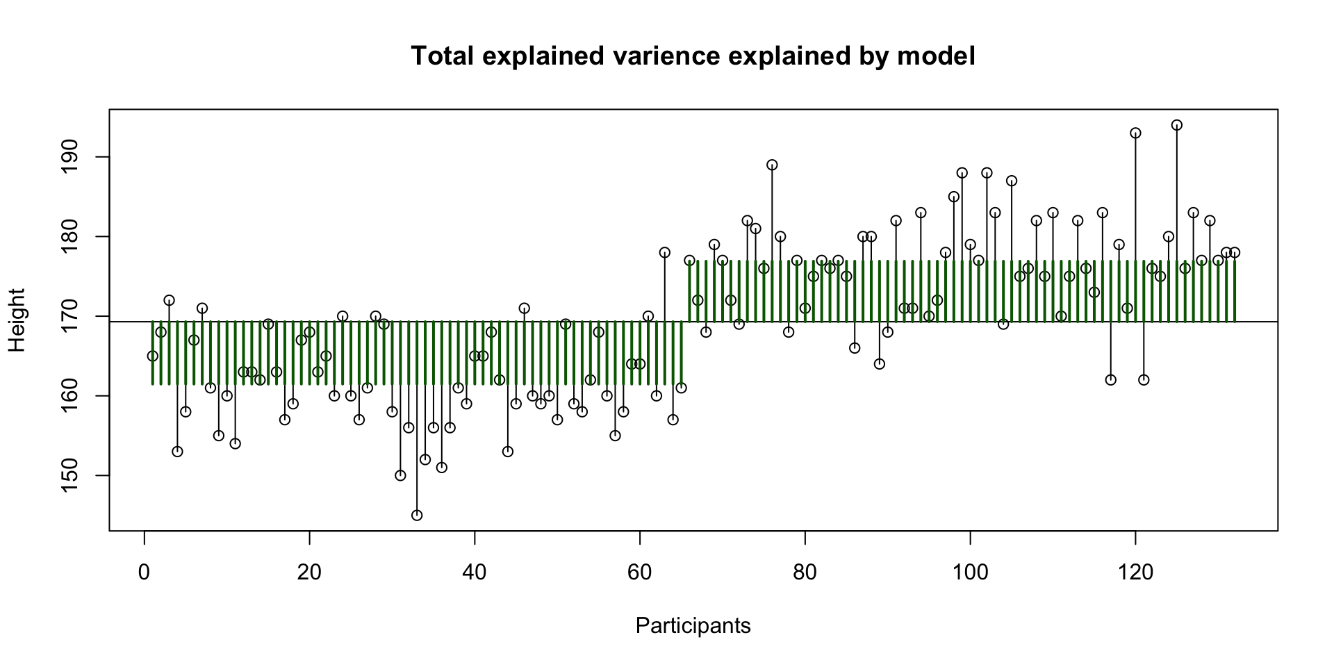
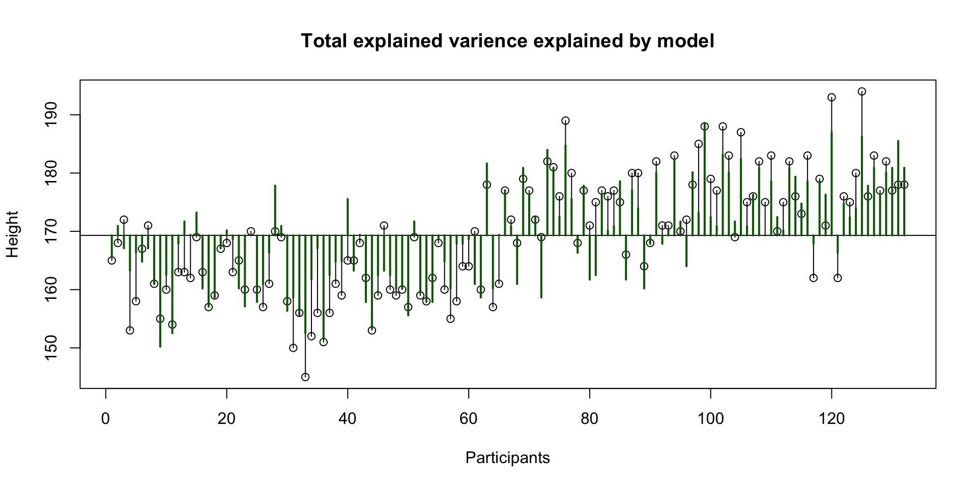
Outcome vs Model
The better the model, the more it is the same as the outcome variable. Hence, they have a high correlation \(r\), and the explained variance \(R^2\) is also high.
\(_i\) is the index number for the data. A row in your data.
\(\beta\) is the true population parameter
\(X\) is your predictor variable
\(\epsilon\) is the error. How much is the model off.
The \(\hat{\phantom{Y}}\) refers to the expected outcome. So, it is the result of the model.
ANOVA as regression
To run an ANOVA as a regression model we need to create dummy variables for each categorical variable that we use. We need \(k - 1\) dummy variables, where \(k\) is the amount of categories.
So, for the categorical variable biological sex, we need 1 dummy.
Dummy variable
Creating a dummy variable means making a new variable in SPSS to turn on that category, and turn all other categories off.
In our case, biological sex has two categories, so we need one dummy. Let’s call our dummy male.
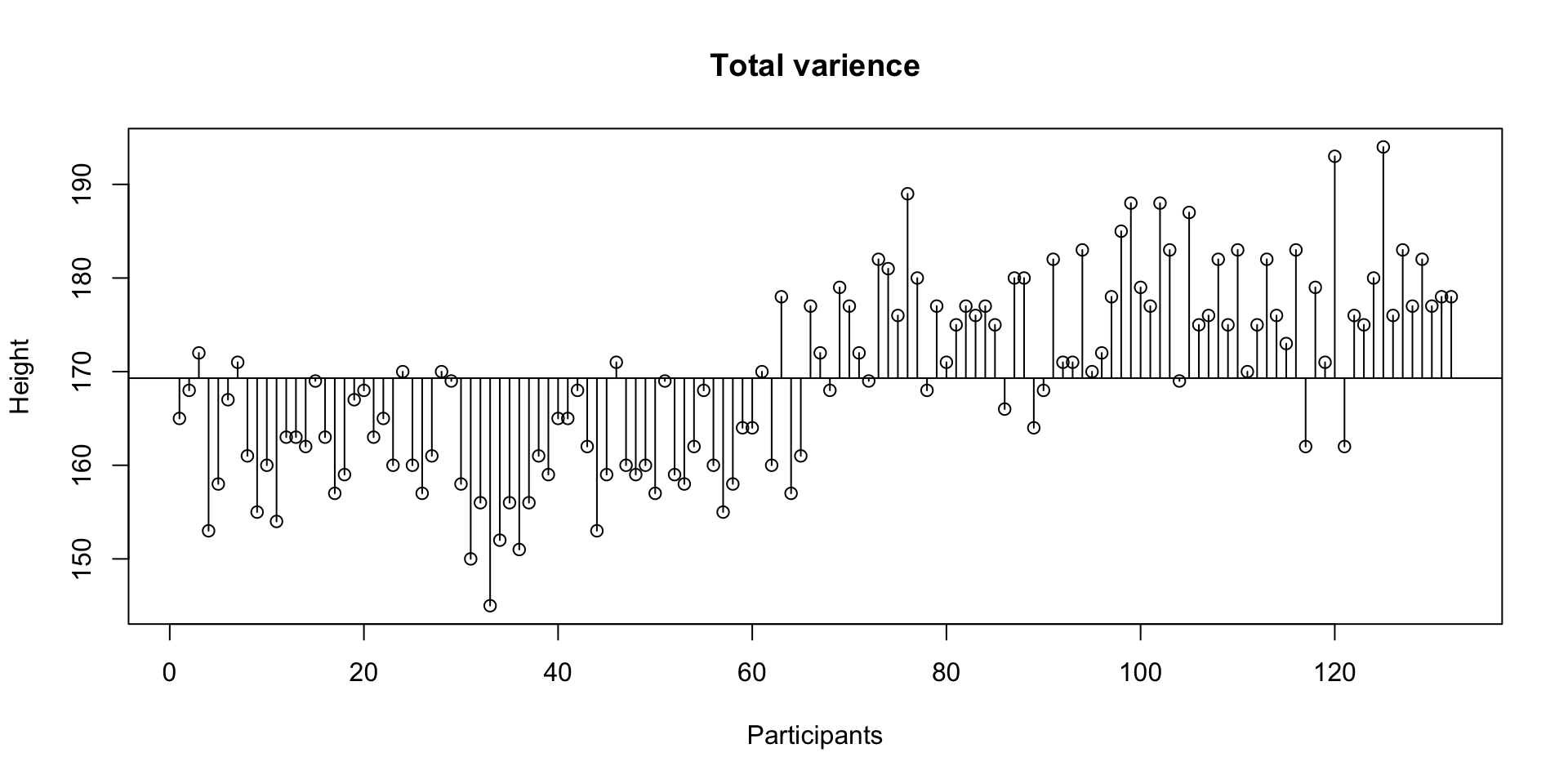
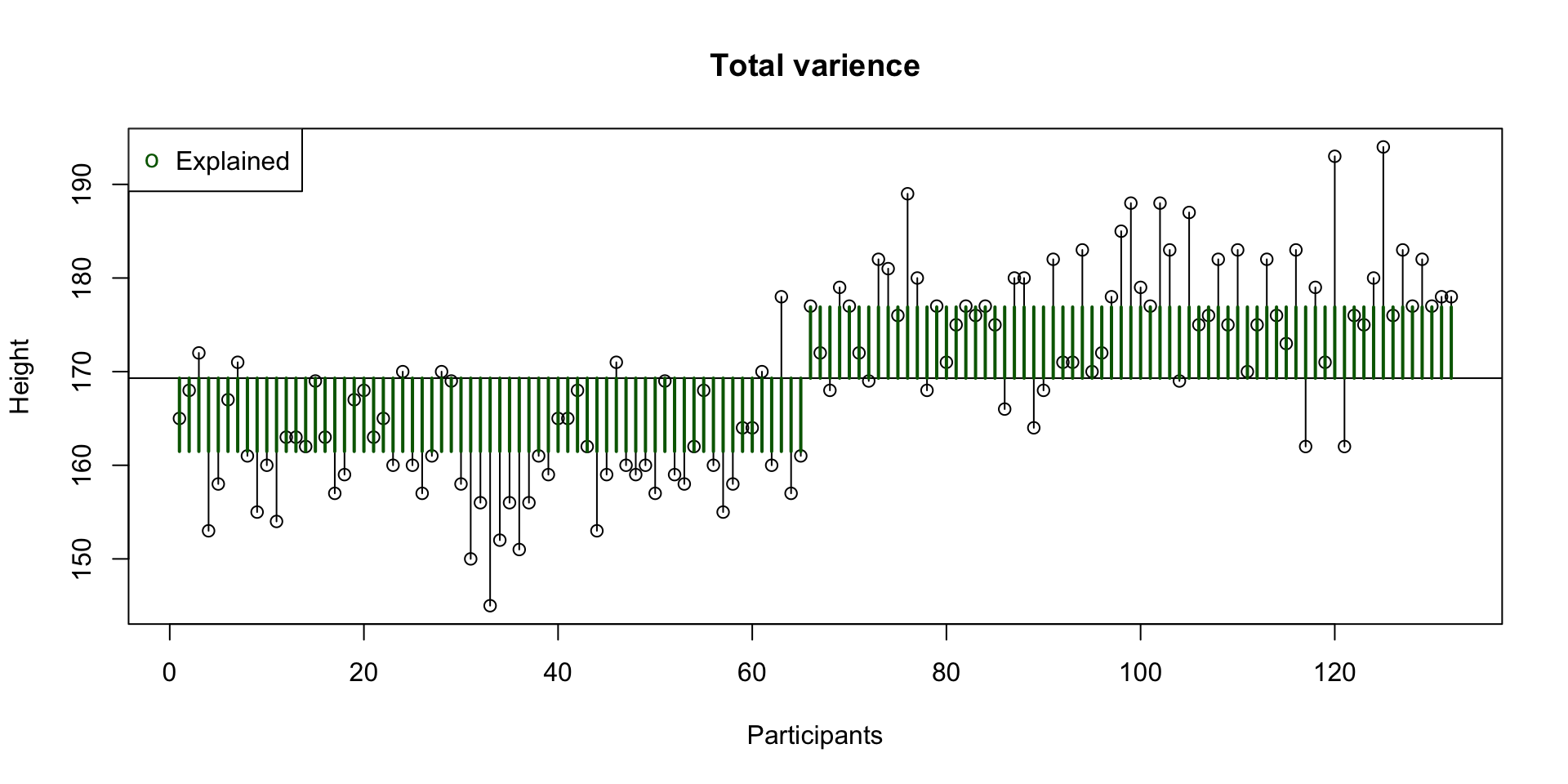
Analysis of Variance Table

Response: height
           Df Sum Sq Mean Sq F value    Pr(>F)
sex         1 7843.4  7843.4  190.64 < 2.2e-16 ***
Residuals 130 5348.5    41.1
---
Signif. codes:  0 '***' 0.001 '**' 0.01 '*' 0.05 '.' 0.1 ' ' 1
F-distribution
Ronald Fisher
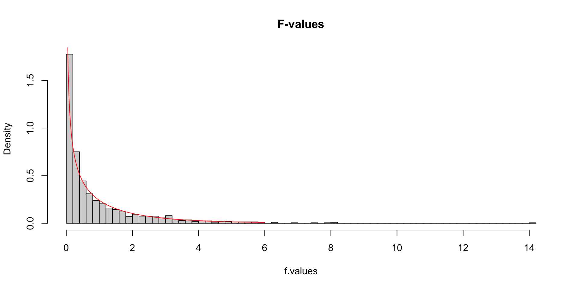
The F-distribution, also known as Snedecor’s F distribution or the Fisher–Snedecor distribution (after Ronald Fisher and George W. Snedecor) is, in probability theory and statistics, a continuous probability distribution. The F-distribution arises frequently as the null distribution of a test statistic, most notably in the analysis of variance; see F-test.
Sir Ronald Aylmer Fisher FRS (17 February 1890 – 29 July 1962), known as R.A. Fisher, was an English statistician, evolutionary biologist, mathematician, geneticist, and eugenicist. Fisher is known as one of the three principal founders of population genetics, creating a mathematical and statistical basis for biology and uniting natural selection with Mendelian genetics.
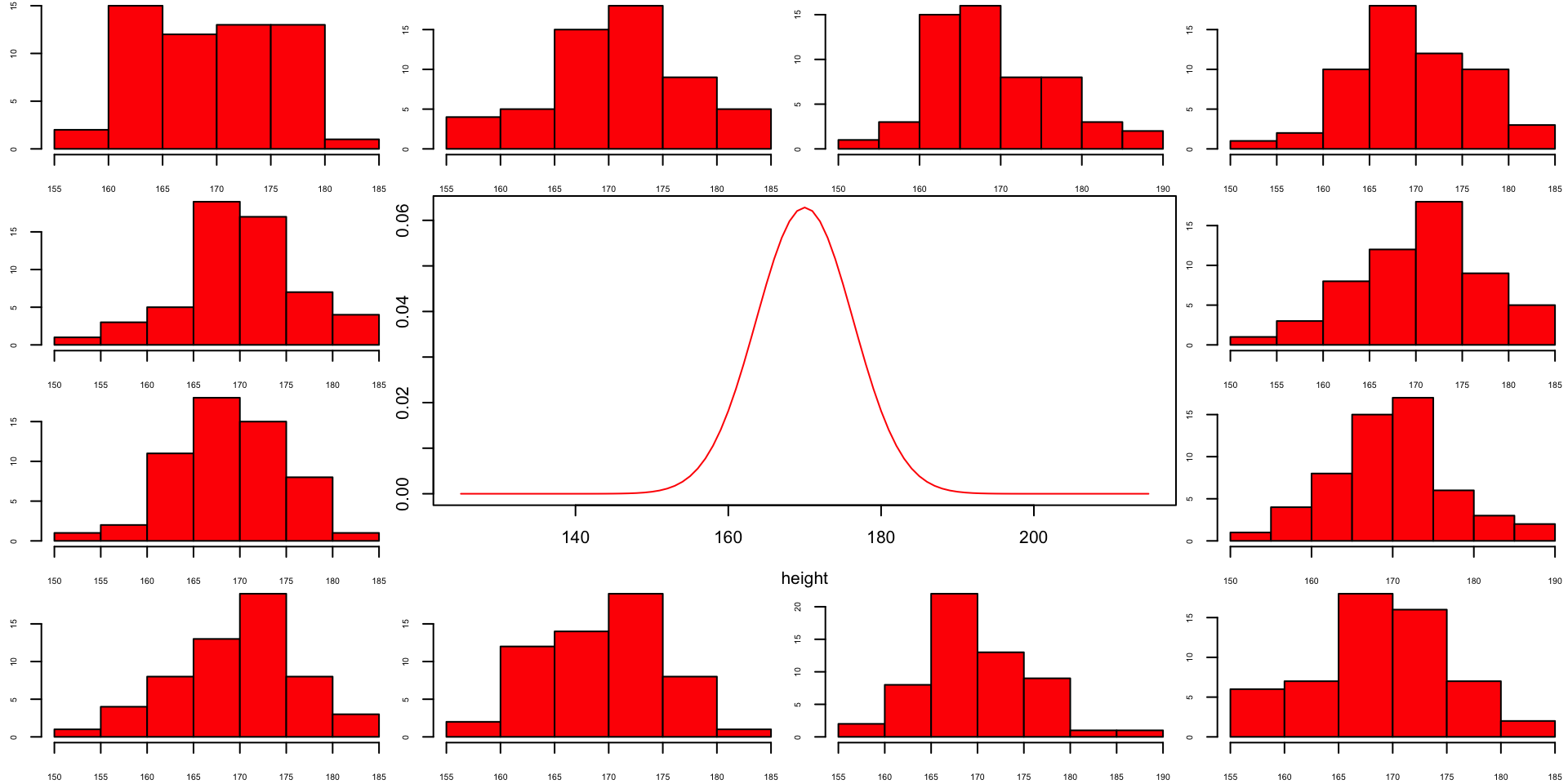
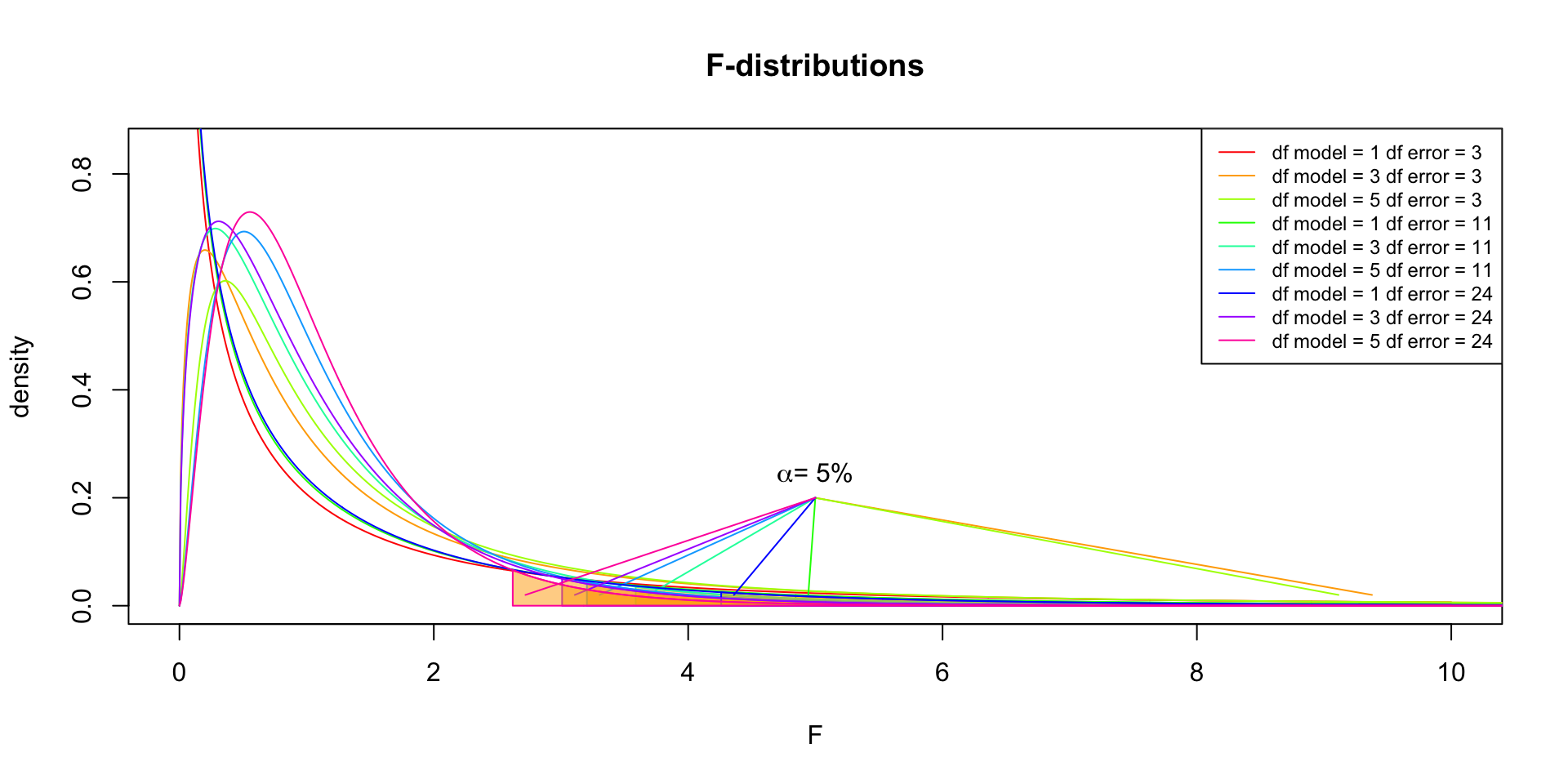
So if the population is normally distributed (assumption of normality) the f-distribution represents the signal to noise ratio given a certain number of samples (\({df}_{model} = k - 1\)) and sample size (\({df}_{error} = N - k\)).
The F-distibution therefore is different for different sample sizes and number of groups.
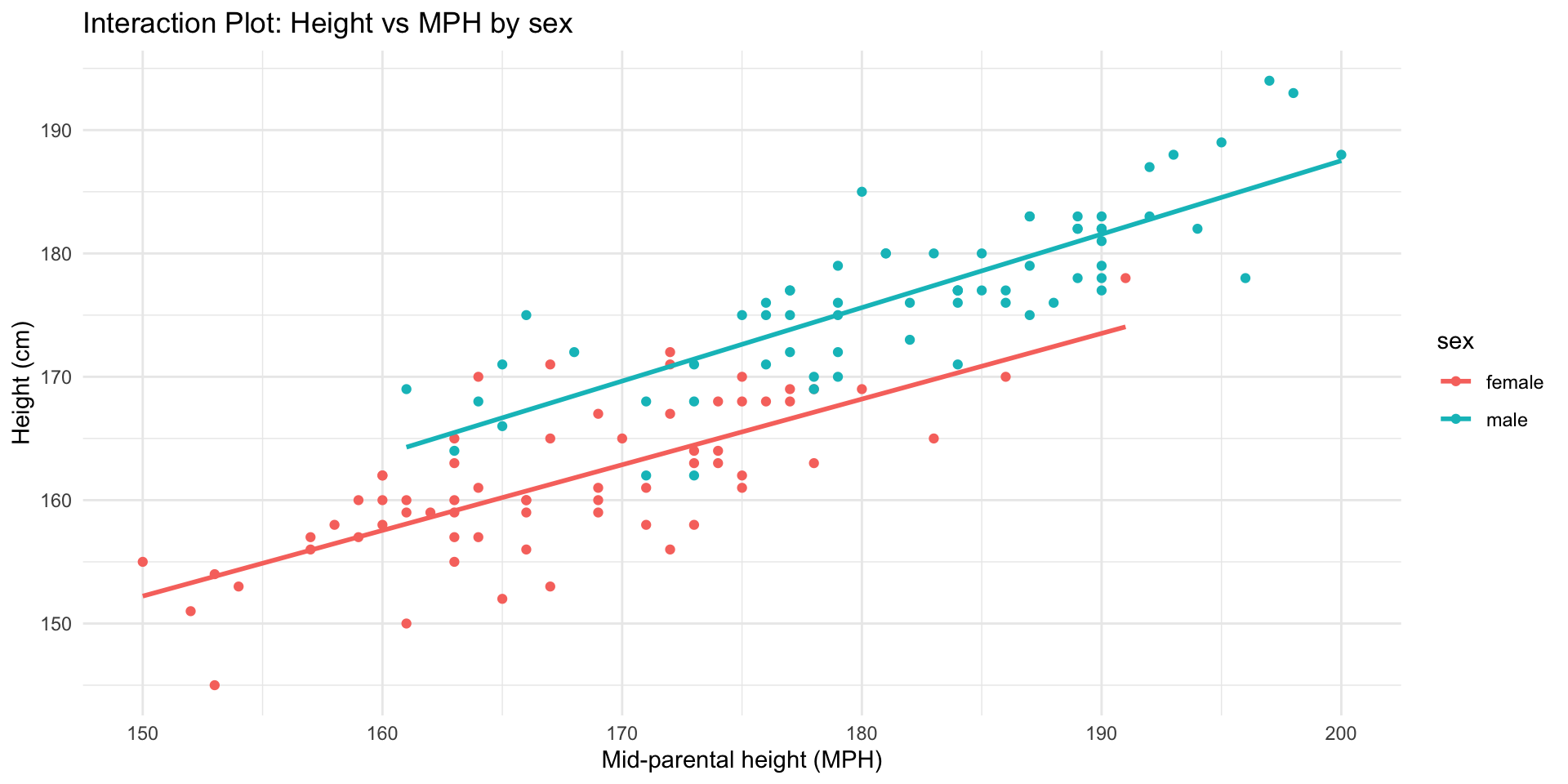
In statistics and regression analysis, moderation occurs when the relationship between two variables depends on a third variable. The third variable is referred to as the moderator variable or simply the moderator. The effect of a moderating variable is characterized statistically as an interaction.
Categorical and continuous predictor
Another good predictor for height is the mid-parental height. That is, the biological sex adjusted average height of both parents.