Alternatives to NHST
The problem with
P-values
There is no problem
The problem with P-values is that they are often misunderstood and misinterpreted. The P-value is the probability of observing a sample statistic as or more extreme as the one obtained, given that the null hypothesis is true. It is NOT the probability that the null hypothesis is true. The P-value is NOT a measure of the strength of the evidence against the null hypothesis.
The misinterpretation is the problem, and not adhering to the Nayman-Pearson paradigm
The dance of the P-value
H0 and HA distribution
G*Power
Determine the required sample size for a desired test power, significance level, and effect size.
G*Power is a tool to compute statistical power analyses for many different \(t\) tests, \(F\) tests, \(\chi^2\) tests, \(z\) tests and some exact tests.

Confidence Interval
The confidence interval is a range of values that is likely to contain the true value of an unknown population parameter. The confidence interval is calculated from a given set of sample data. The confidence interval is used to express the uncertainty associated with a sample estimate of a population parameter.
We use the standard error to calculate the lower and upper limit of the confidence interval.
Standard Error
95% confidence interval
\[SE = \frac{\text{Standard deviation}}{\text{Square root of sample size}} = \frac{s}{\sqrt{n}}\]
- Lowerbound = \(\bar{x} - 1.96 \times SE\)
- Upperbound = \(\bar{x} + 1.96 \times SE\)

Plot CI

5 out of 100 samples

Common Misinterpretations
Confidence intervals and levels are frequently misunderstood, and published studies have shown that even professional scientists often misinterpret them (Wikipedia, 2024)
Hoekstra, Morey, Rouder, & Wagenmakers (2014) administerred the following questionair to 120 researchers.
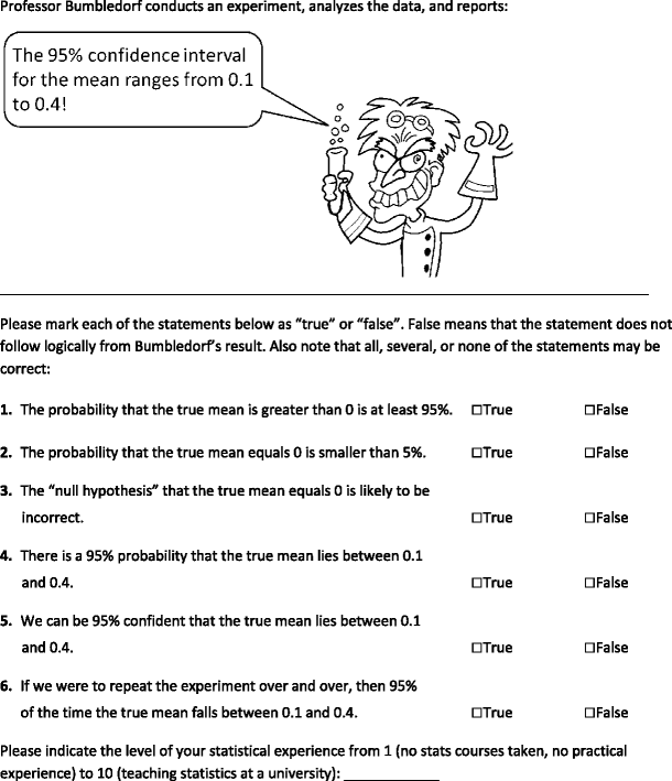
All of the statements are false
Researcher don’t know
| #True | First-Year Students (n = 442) | Master Students (n = 34) | Researchers (n = 118) |
|---|---|---|---|
| 0 | 2% | 0% | 3% |
| 1 | 6% | 24% | 9% |
| 2 | 14% | 18% | 14% |
| 3 | 26% | 15% | 25% |
| 4 | 30% | 12% | 22% |
| 5 | 15% | 21% | 16% |
| 6 | 7% | 12% | 11% |
Conclusion
Use both NHST and confidence intervals
Example

We also studied the validity by comparing the mean ability ratings of children in different grades. We expected a positive relation between grade and ability. Figure 5 shows the average ability rating for each grade and domain. As expected, children in older age groups had a higher rating than children in younger age groups. In all four domains, there is an overall significant effect of grade: addition \(F(5,1456)=1091.4,p<.01,\omega^2=.78\), subtraction \(F(5,1363)=780.5,p<.01,\omega^2=.74\), multiplication \(F(5,1215)=409.6,p<.01,\omega^2=.62\), and \(F(5,973)=223.31,p<.01,\omega^2=.53\) for division. Levene’s tests show differences in variances for the domains multiplication and division. However, the non-parametric Kruskal-Wallis tests also show significant differences for these domains: \(\chi^2(5)=753.28,p<.01\) for multiplication and \(\chi^2(5)=505.17,p<.01\) for division. For all domains, post hoc analyses show significant differences between all grades, except for the differences between grades five and six (Klinkenberg, Straatemeier, & van der Maas, 2011).
End
Contact
