layout(matrix(c(2:6,1,1,7:8,1,1,9:13), 4, 4))
n = 56 # Sample size
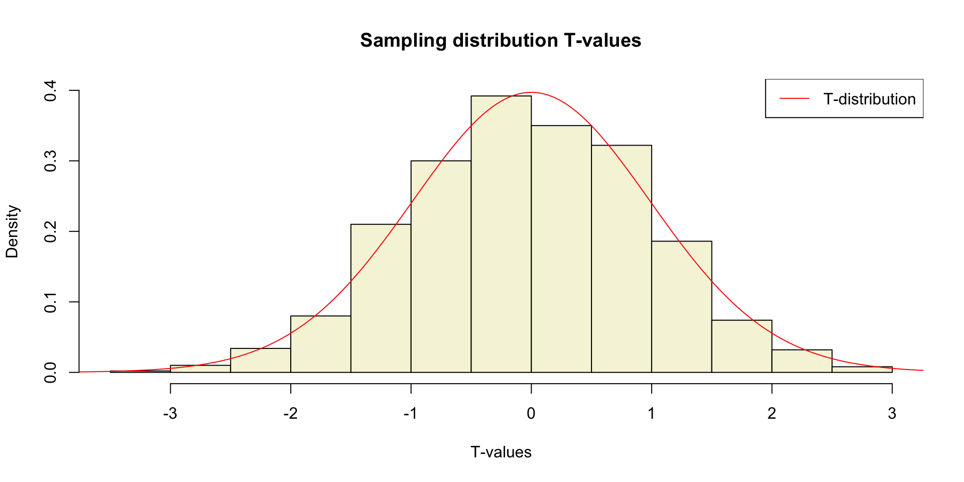
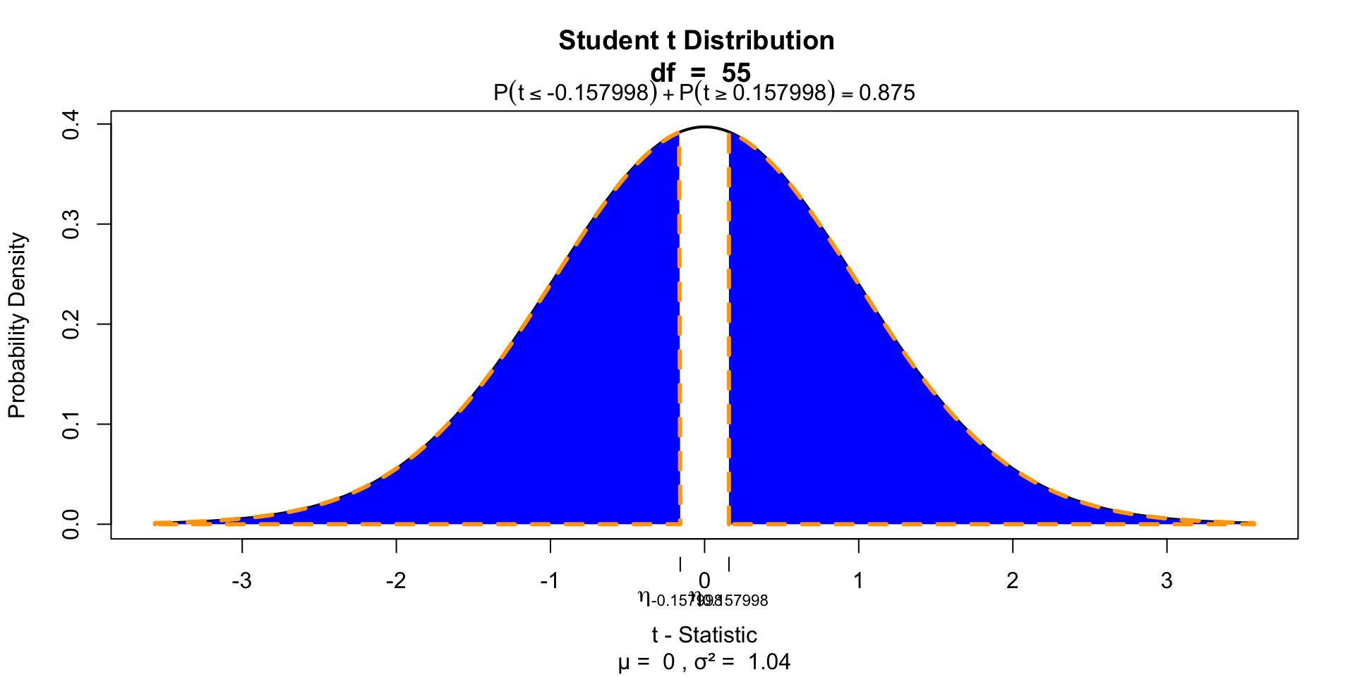
df = n - 1 # Degrees of freedom
mu = 120
sigma = 15
IQ = seq(mu-45, mu+45, 1)
par(mar=c(4,2,2,0))
plot(IQ, dnorm(IQ, mean = mu, sd = sigma), type='l', col="red", main = "Population Distribution")
n.samples = 12
for(i in 1:n.samples) {
par(mar=c(2,2,2,0))
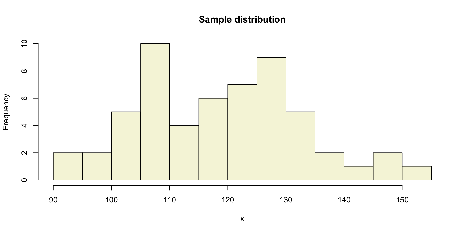
hist(rnorm(n, mu, sigma), main="Sample Distribution", cex.axis=.5, col="beige", cex.main = .75)
}T-Distribution NHST
9/18/23
IQ next to you

http://goo.gl/T6Lo2s
Gosset

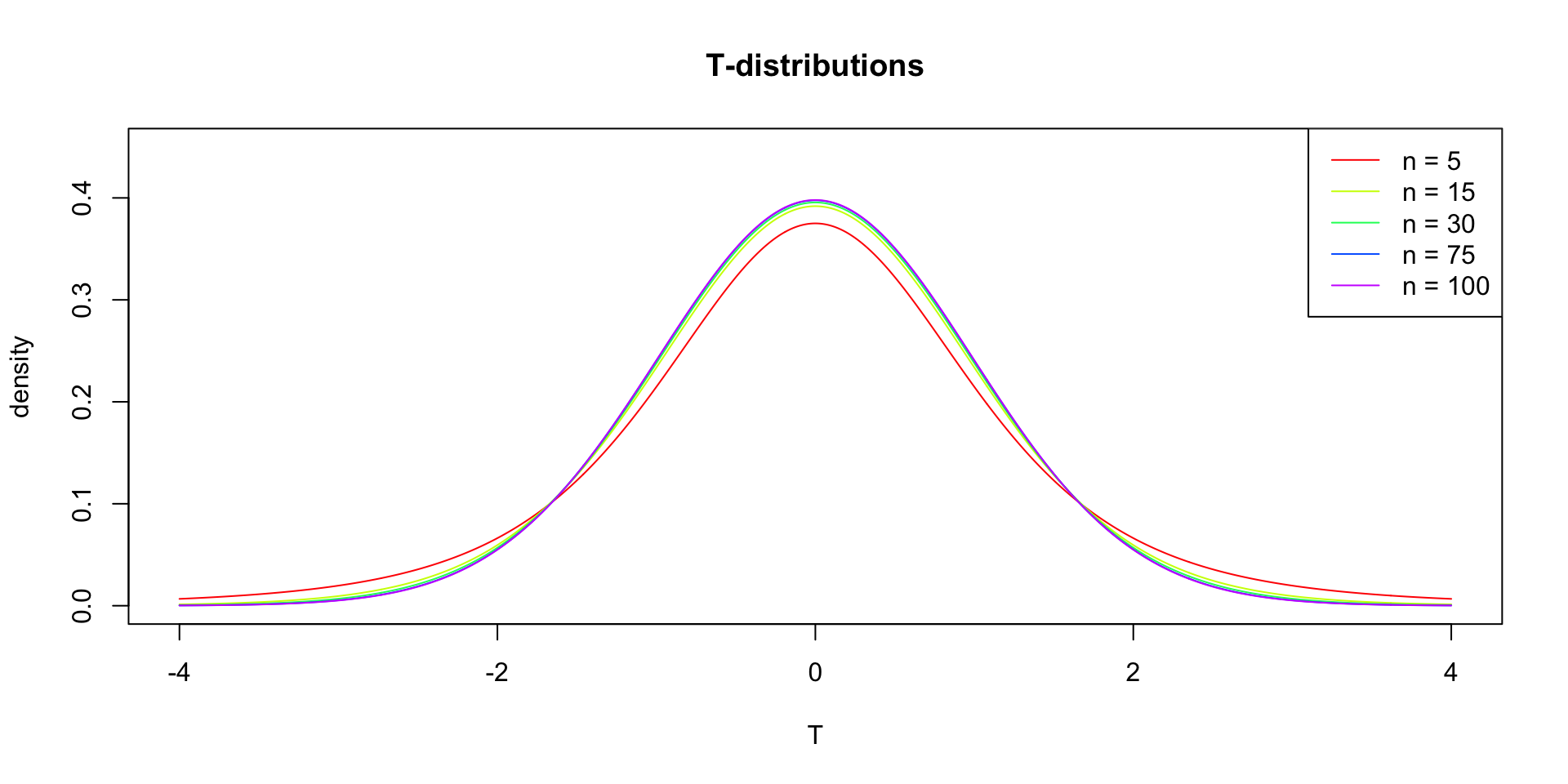
In probability and statistics, Student’s t-distribution (or simply the t-distribution) is any member of a family of continuous probability distributions that arises when estimating the mean of a normally distributed population in situations where the sample size is small and population standard deviation is unknown.
In the English-language literature it takes its name from William Sealy Gosset’s 1908 paper in Biometrika under the pseudonym “Student”. Gosset worked at the Guinness Brewery in Dublin, Ireland, and was interested in the problems of small samples, for example the chemical properties of barley where sample sizes might be as low as 3.
Source: Wikipedia
Population distribution
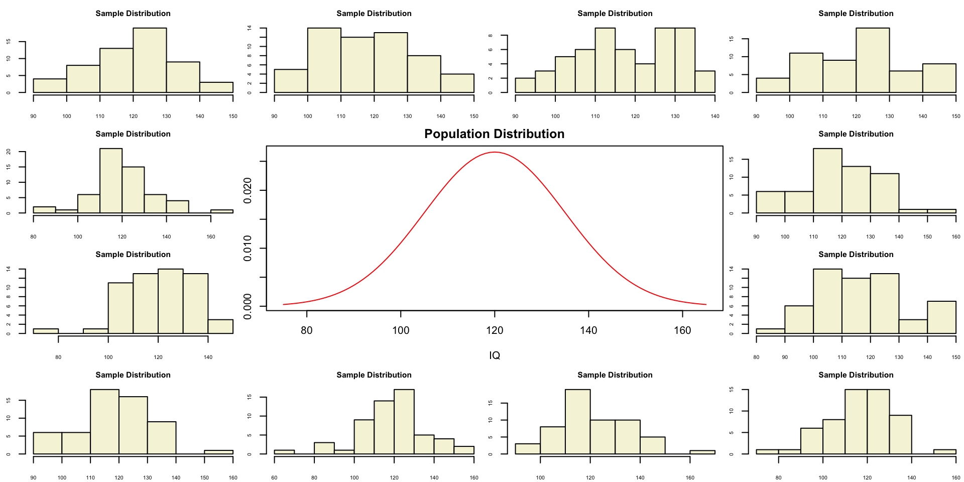
A sample
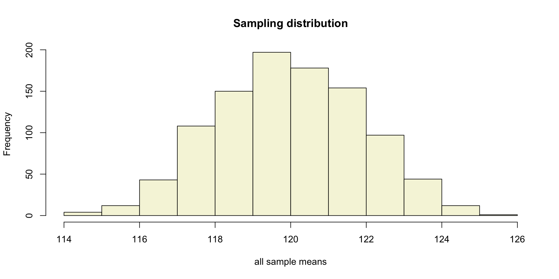
Sampling distribution
of the mean
Sampling distribution t-values
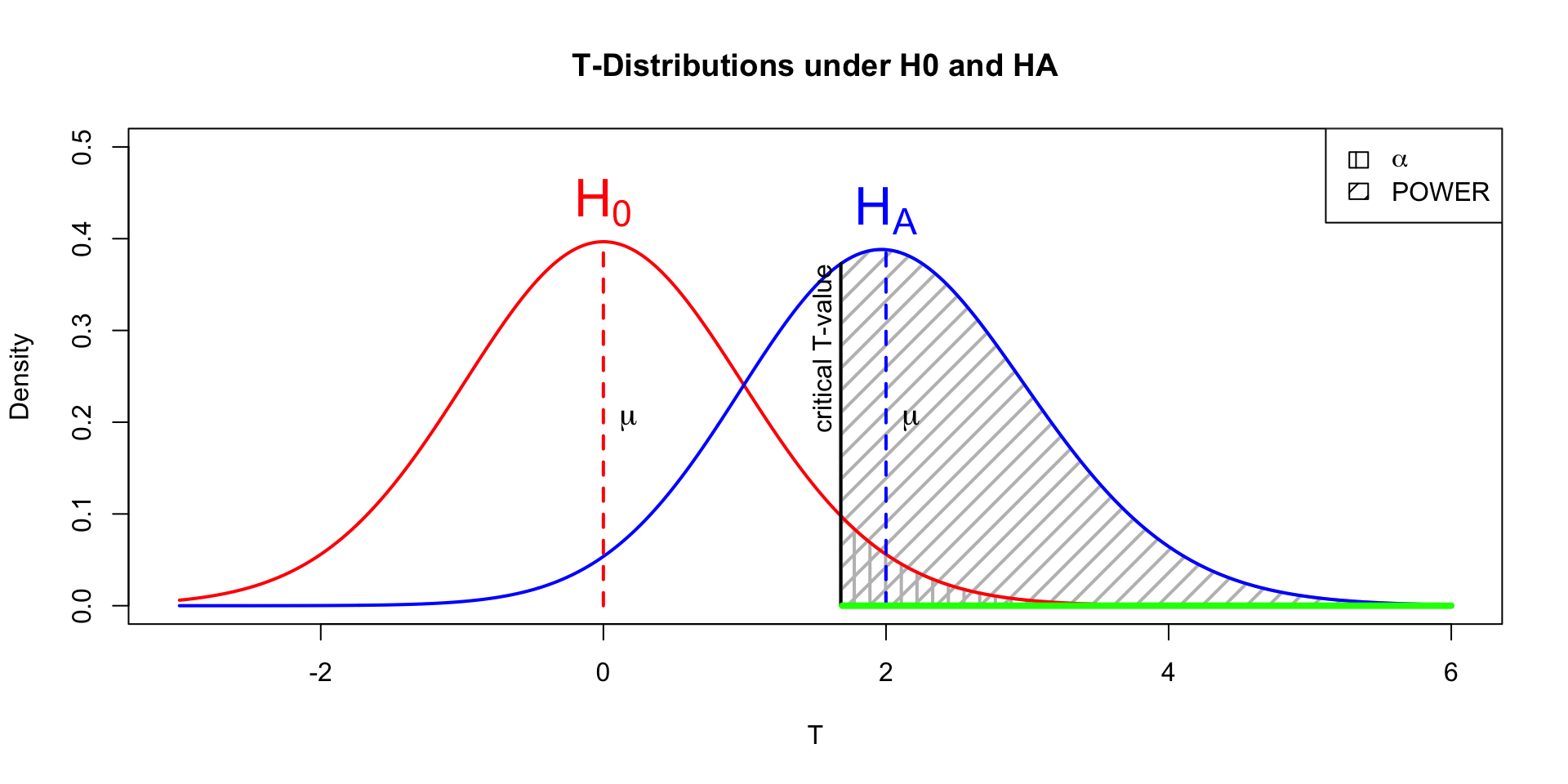
Power
- Strive for 80%
- Based on known effect size
- Calculate number of subjects needed
- Use G*Power to calculate

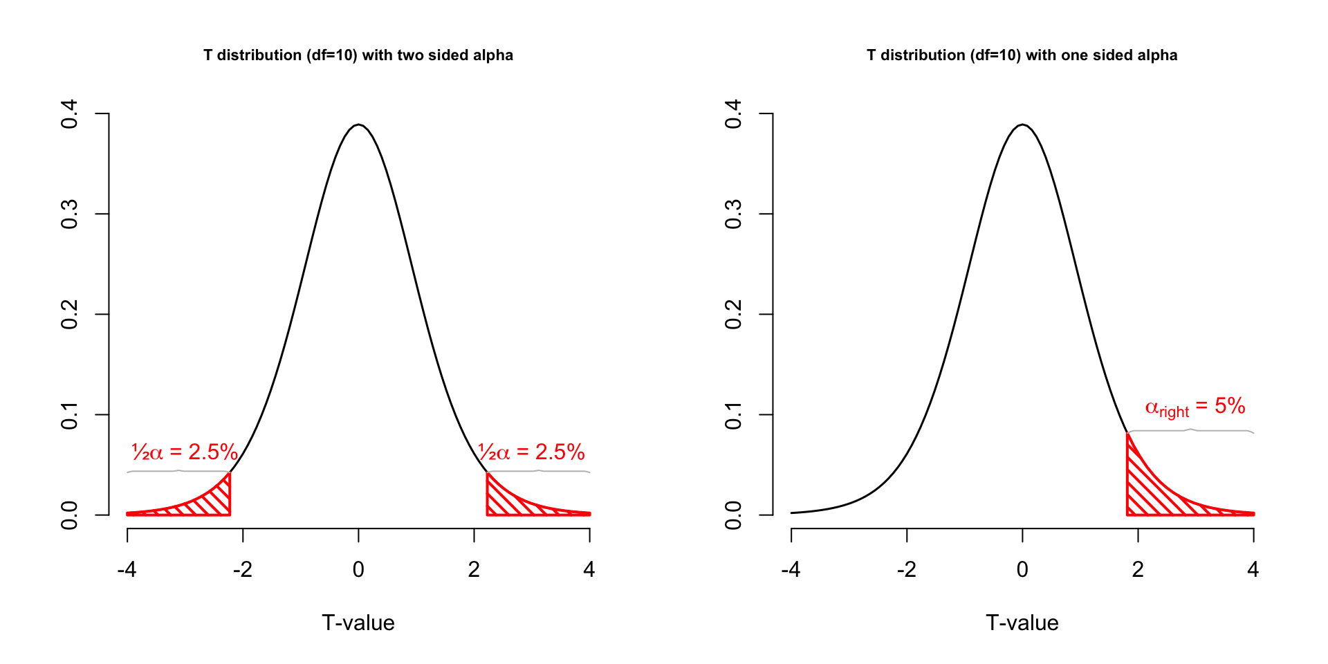
Alpha Power
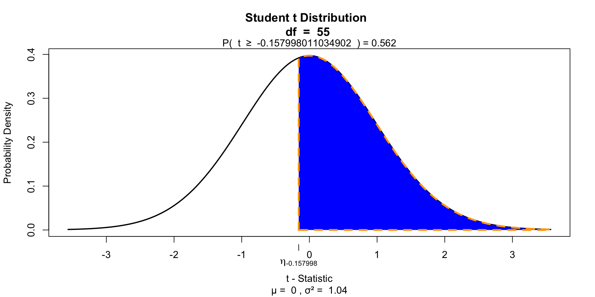
P-value one sided
Finally we have to calculate our p-value for which we need the degrees of freedom \(df = n - 1\) to determine the shape of the t-distribution.
P-value two sided
Contact

![]()