T-Distribution NHST

Author

Affiliation

Klinkenberg

University of Amsterdam

Published

September 18, 2023

IQ next to you

http://goo.gl/T6Lo2s

Models

\[\text{outcome} = \text{model} + \text{error}\]

T-distribution

Gosset

In probability and statistics, Student’s t-distribution (or simply the t-distribution) is any member of a family of continuous probability distributions that arises when estimating the mean of a normally distributed population in situations where the sample size is small and population standard deviation is unknown.

In the English-language literature it takes its name from William Sealy Gosset’s 1908 paper in Biometrika under the pseudonym “Student”. Gosset worked at the Guinness Brewery in Dublin, Ireland, and was interested in the problems of small samples, for example the chemical properties of barley where sample sizes might be as low as 3.

Source: Wikipedia

Population distribution

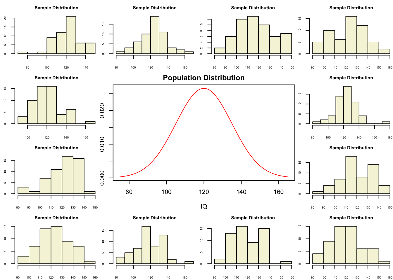
layout(matrix(c(2:6,1,1,7:8,1,1,9:13), 4, 4))

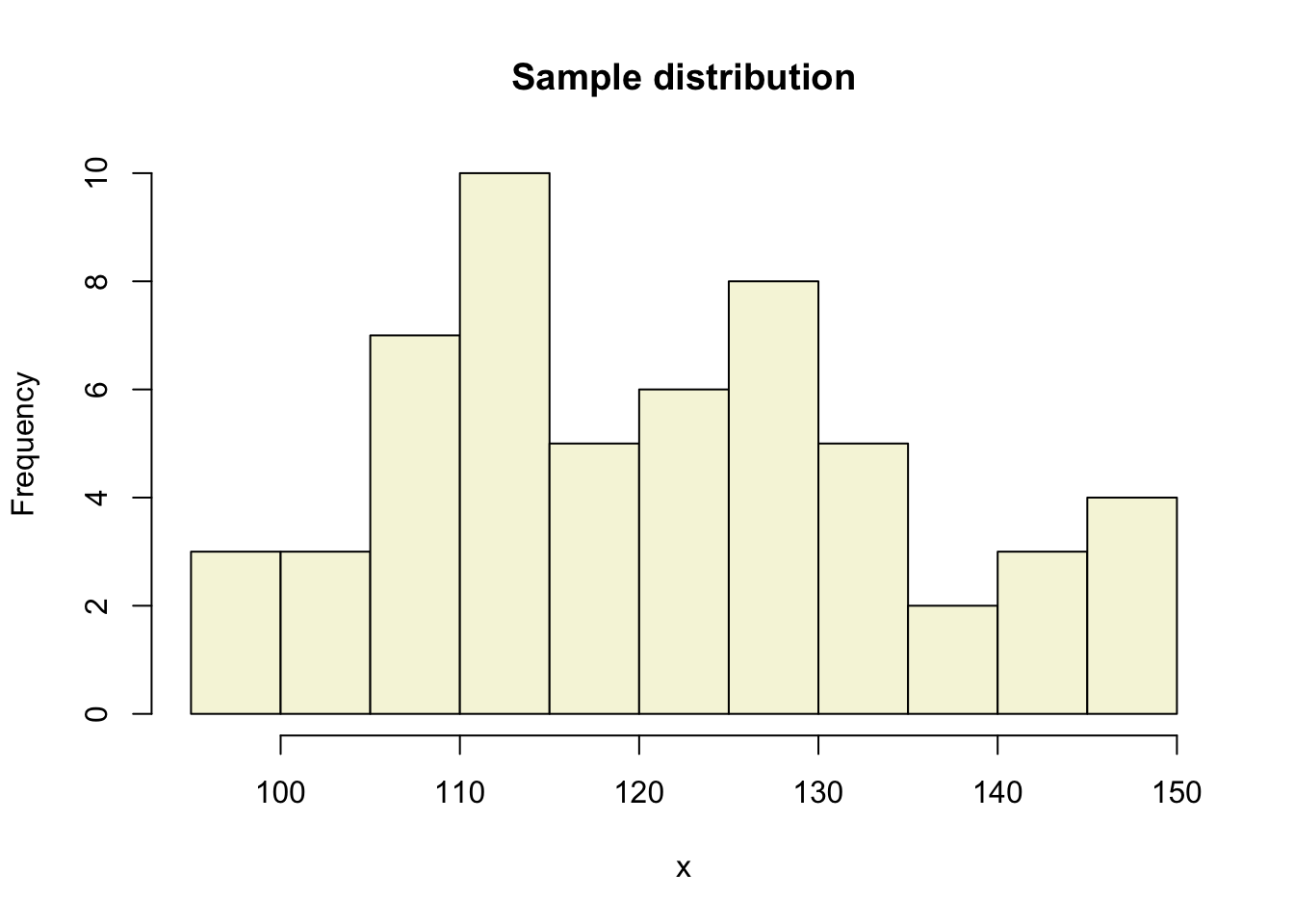
n  = 56    # Sample size
df = n - 1 # Degrees of freedom

mu    = 120
sigma = 15

IQ = seq(mu-45, mu+45, 1)

par(mar=c(4,2,2,0))  
plot(IQ, dnorm(IQ, mean = mu, sd = sigma), type='l', col="red", main = "Population Distribution")

n.samples = 12

for(i in 1:n.samples) {
  
  par(mar=c(2,2,2,0))  
  hist(rnorm(n, mu, sigma), main="Sample Distribution", cex.axis=.5, col="beige", cex.main = .75)
  
}

A sample

Let’s take a larger sample from our normal population.

x = rnorm(n, mu, sigma); x

 [1] 107.98215 127.93494 116.01242 108.91514 127.76013 119.74741 138.60983
 [8] 123.02093 113.26615 111.89251 132.81938 127.20798 114.49846 114.87101
[15] 118.09146 139.39516 130.97532 129.93712 147.91924 110.08536 102.63386
[22]  95.29534 128.19719 113.02769 140.12850 127.61447 121.59205 124.10600
[29] 111.79133 149.77465  98.74904  99.18328 146.31027 104.22330 109.29647
[36] 140.64673 124.78663 123.00386 144.19090 129.62958 113.54822 112.56255
[43] 122.59632 130.08247 109.04033 103.28132 105.44416 119.56329 131.59294
[50] 130.93613 148.82209 109.21116 107.74051 125.75232 113.68687 119.53250

hist(x, main = "Sample distribution", col = "beige", breaks = 15)
text(80, 10, round(mean(x),2))

More samples

let’s take more samples.

n.samples     = 1000
mean.x.values = vector()
sd.x.values   = vector()
se.x.values   = vector()

for(i in 1:n.samples) {
  x = rnorm(n, mu, sigma)
  mean.x.values[i] = mean(x)
  se.x.values[i]   = (sd(x) / sqrt(n))
  sd.x.values[i]   = sd(x)
}

Mean and SE for all samples

head(cbind(mean.x.values, se.x.values))

     mean.x.values se.x.values
[1,]      118.5294    1.721504
[2,]      118.8394    2.315007
[3,]      119.3210    2.045235
[4,]      118.2852    1.986011
[5,]      119.7502    1.876294
[6,]      118.9140    1.797314

Sampling distribution

of the mean

T-statistic

\[T_{n-1} = \frac{\bar{x}-\mu}{SE_x} = \frac{\bar{x}-\mu}{s_x / \sqrt{n}}\]

So the t-statistic represents the deviation of the sample mean \(\bar{x}\) from the population mean \(\mu\), considering the sample size, expressed as the degrees of freedom \(df = n - 1\)

t-value

\[T_{n-1} = \frac{\bar{x}-\mu}{SE_x} = \frac{\bar{x}-\mu}{s_x / \sqrt{n}}\]

t = (mean(x) - mu) / (sd(x) / sqrt(n))
t

[1] -0.3667779

Calculate t-values

\[T_{n-1} = \frac{\bar{x}-\mu}{SE_x} = \frac{\bar{x}-\mu}{s_x / \sqrt{n}}\]

t.values = (mean.x.values - mu) / se.x.values

tail(cbind(mean.x.values, mu, se.x.values, t.values))

        mean.x.values  mu se.x.values   t.values
 [995,]      119.4467 120    1.763711 -0.3136863
 [996,]      119.0913 120    1.995133 -0.4554445
 [997,]      122.7020 120    2.010682  1.3438434
 [998,]      119.3597 120    1.647172 -0.3887262
 [999,]      119.9545 120    2.000003 -0.0227549
[1000,]      119.2847 120    1.950359 -0.3667779

Sampling distribution t-values

T-distribution

So if the population is normaly distributed (assumption of normality) the t-distribution represents the deviation of sample means from the population mean (\(\mu\)), given a certain sample size (\(df = n - 1\)).

The t-distibution therefore is different for different sample sizes and converges to a standard normal distribution if sample size is large enough.

The t-distribution is defined by:

\[\textstyle\frac{\Gamma \left(\frac{\nu+1}{2} \right)} {\sqrt{\nu\pi}\,\Gamma \left(\frac{\nu}{2} \right)} \left(1+\frac{x^2}{\nu} \right)^{-\frac{\nu+1}{2}}\!\]

where \(\nu\) is the number of degrees of freedom and \(\Gamma\) is the gamma function.

Source: wikipedia