F-Distribution and factorial ANOVA

Author

Affiliation

Klinkenberg

University of Amsterdam

Published

September 25, 2023

F-distribution

Ronald Fisher

The F-distribution, also known as Snedecor’s F distribution or the Fisher–Snedecor distribution (after Ronald Fisher and George W. Snedecor) is, in probability theory and statistics, a continuous probability distribution. The F-distribution arises frequently as the null distribution of a test statistic, most notably in the analysis of variance; see F-test.

Wikipedia

Sir Ronald Aylmer Fisher FRS (17 February 1890 – 29 July 1962), known as R.A. Fisher, was an English statistician, evolutionary biologist, mathematician, geneticist, and eugenicist. Fisher is known as one of the three principal founders of population genetics, creating a mathematical and statistical basis for biology and uniting natural selection with Mendelian genetics.

Wikipedia

Analysing variance

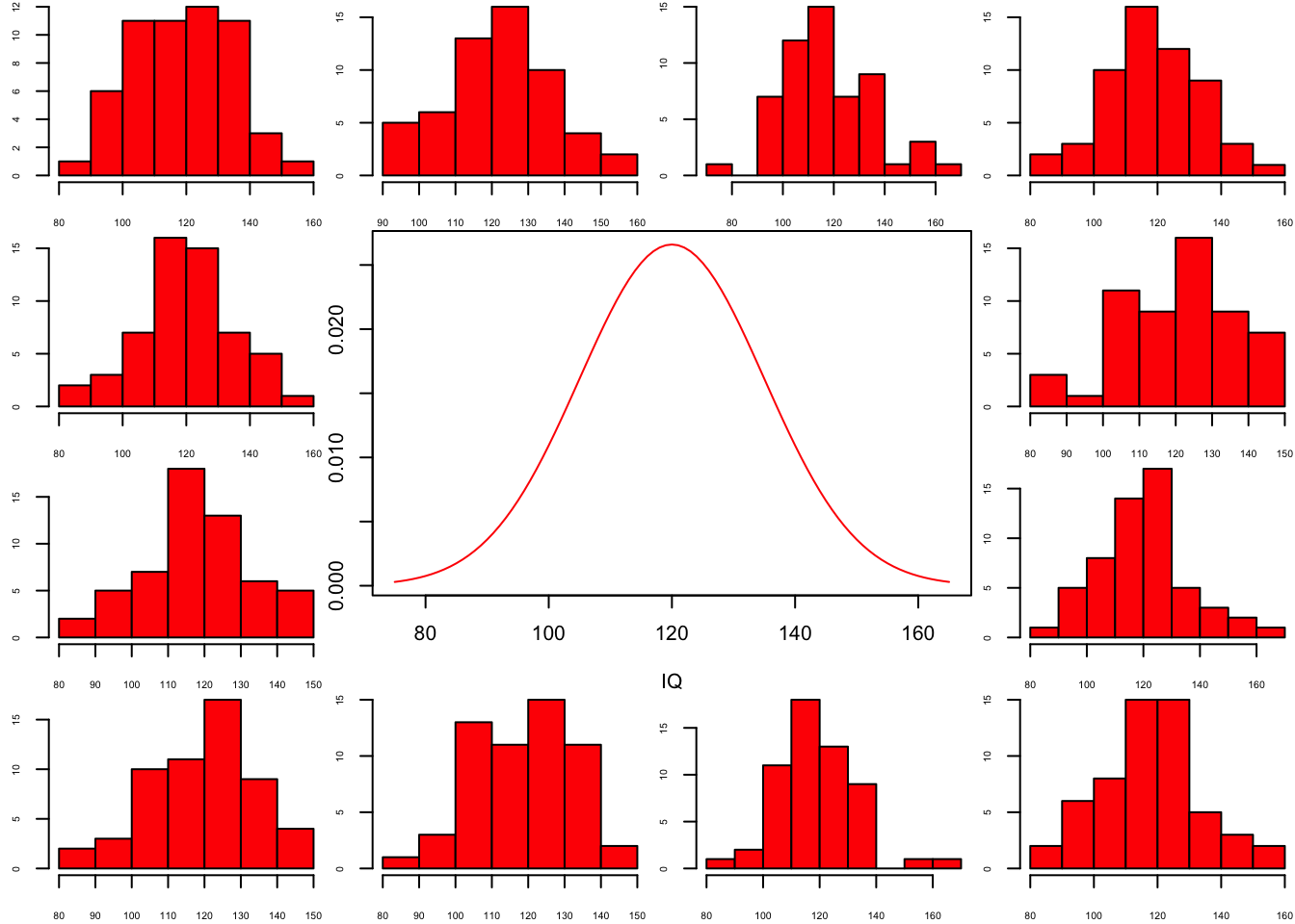
Decomposing variance example of height for males and females.

Population distribution

layout(matrix(c(2:6,1,1,7:8,1,1,9:13), 4, 4))

n  = 56    # Sample size
df = n - 1 # Degrees of freedom

mu    = 120
sigma = 15

IQ = seq(mu-45, mu+45, 1)

par(mar=c(4,2,0,0))  
plot(IQ, dnorm(IQ, mean = mu, sd = sigma), type='l', col="red")

n.samples = 12

for(i in 1:n.samples) {
  
  par(mar=c(2,2,0,0))  
  hist(rnorm(n, mu, sigma), main="", cex.axis=.5, col="red")
  
}

F-statistic

\[F = \frac{{MS}_{model}}{{MS}_{error}} = \frac{\text{between group var.}}{\text{within group var.}} = \frac{{SIGNAL}}{{NOISE}}\]

The \(F\)-statistic represents a signal to noise ratio by defiding the model variance component by the error variance component.

A samples

Let’s take two sample from our normal population and calculate the F-value.

x.1 = rnorm(n, mu, sigma)
x.2 = rnorm(n, mu, sigma)

\[F = \frac{{MS}_{model}}{{MS}_{error}} = \frac{{SIGNAL}}{{NOISE}} = \frac{{522.11}}{{296.77}} = 1.76\]

More samples

let’s take more samples and calculate the F-value every time.

n.samples = 1000

f.values = vector()

for(i in 1:n.samples) {
  
  x.1 = rnorm(n, mu, sigma); x.1
  x.2 = rnorm(n, mu, sigma); x.2

  data <- data.frame(group = rep(c("s1", "s2"), each=n), score = c(x.1,x.2))
    
  f.values[i] = summary(aov(lm(score ~ group, data)))[[1]]$F[1]

}

k = 2
N = 2*n

df.model = k - 1
df.error = N - k

hist(f.values, freq = FALSE, main="F-values", breaks=100)
F = seq(0, 6, .01)
lines(F, df(F,df.model, df.error), col = "red")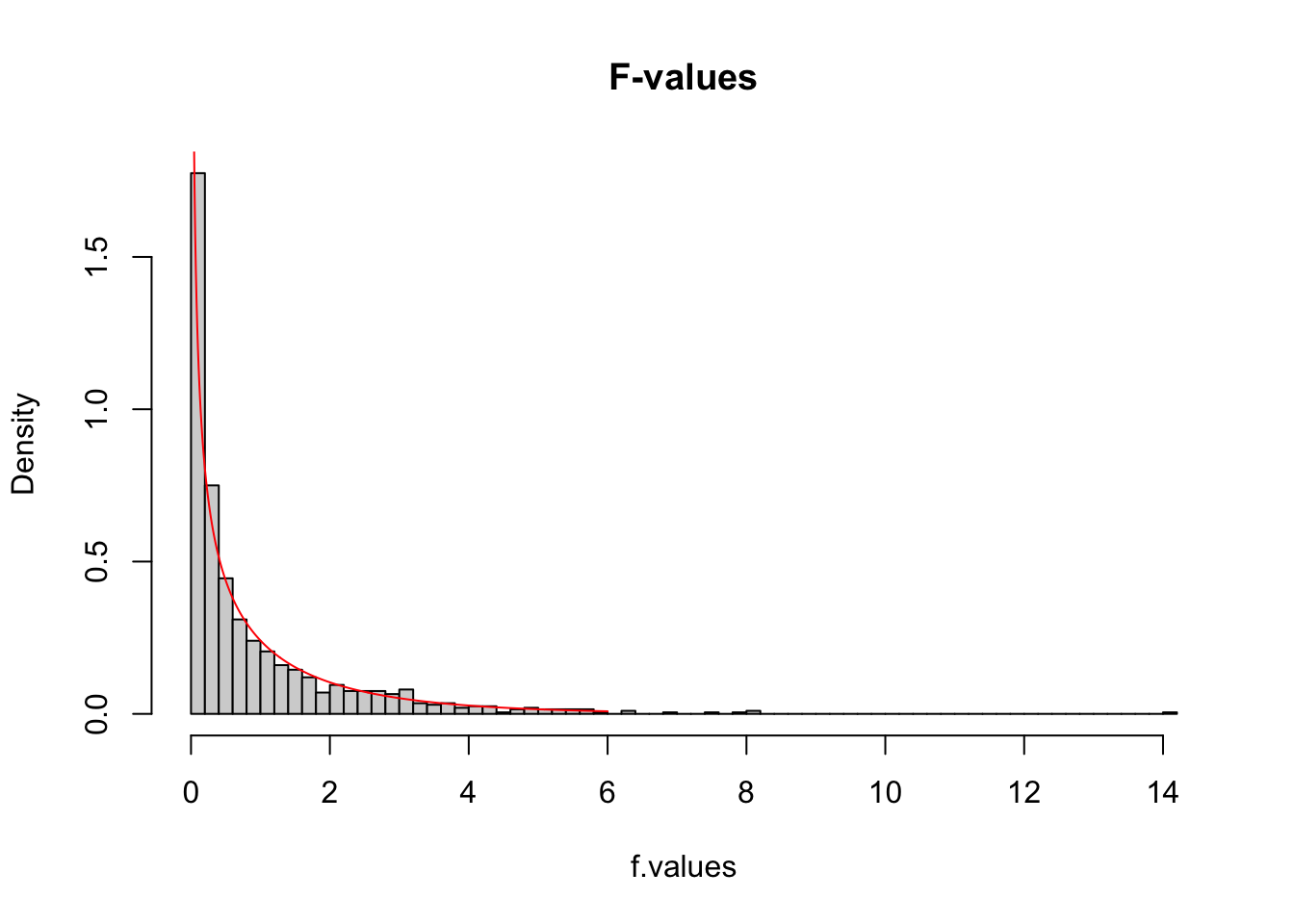

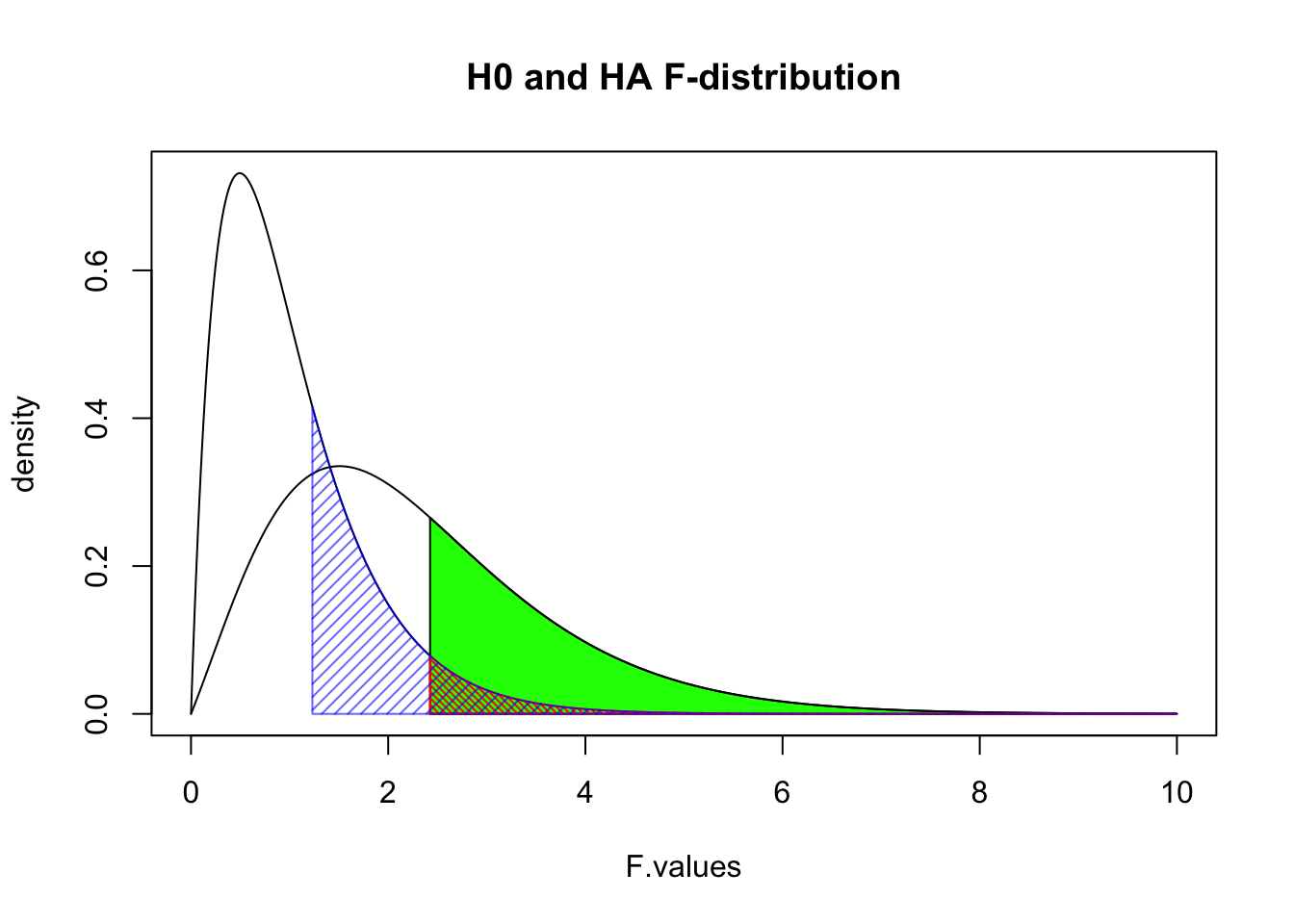
F-distribution

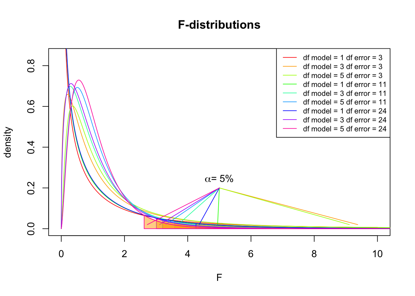
So if the population is normally distributed (assumption of normality) the f-distribution represents the signal to noise ratio given a certain number of samples (\({df}_{model} = k - 1\)) and sample size (\({df}_{error} = N - k\)).

The F-distibution therefore is different for different sample sizes and number of groups.

\[\frac{\sqrt{\frac{(d_1x)^{d_1}\,\,d_2^{d_2}} {(d_1x+d_2)^{d_1+d_2}}}} {x\operatorname{B}\left(\frac{d_1}{2},\frac{d_2}{2}\right)}\]

F-distribution

Independent factorial ANOVA

Two or more independent variables with two or more categories. One dependent variable.

Independent factorial ANOVA

The independent factorial ANOVA analyses the variance of multiple independent variables (Factors) with two or more categories.

Effects and interactions/moderation:

1 dependent/outcome variable
2 or more independent/predictor variables
- 2 or more cat./levels

Assumptions

Continuous variable
Random sample
Normaly distributed
- Shapiro-Wilk test
Equal variance within groups
- Levene’s test

Example

In this example we will look at the amount of accidents in a car driving simulator while subjects where given varying doses of speed and alcohol.

Dependent variable
- Accidents
Independent variables
- Speed
  - None
  - Small
  - Large
- Alcohol
  - None
  - Small
  - Large

person	alcohol	speed	accidents
1	1	1	0
2	1	2	2
3	1	3	4
4	2	1	6
5	2	2	8
6	2	3	10
7	3	1	12
8	3	2	14
9	3	3	16

Data

Effects

Total
- \(F = \frac{{MS}_{model}}{{MS}_{error}}\)
Main effects
- \(F = \frac{{MS}_{goup A}}{{MS}_{error}}\)
- \(F = \frac{{MS}_{goup B}}{{MS}_{error}}\)
Interaction/moderation
- \(F = \frac{{MS}_{A \times B}}{{MS}_{error}}\)

\(MS = \text{Mean Squares}\)

\(MS = \frac{SS}{df}\)

\(SS = \text{Sums of Squares}\)

\(df = \text{degrees of freedom}\)

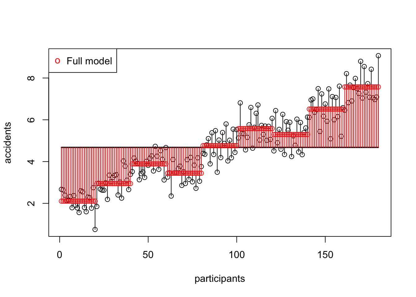
SS model

\(\text{SS}_\text{model} = 494.22048\)

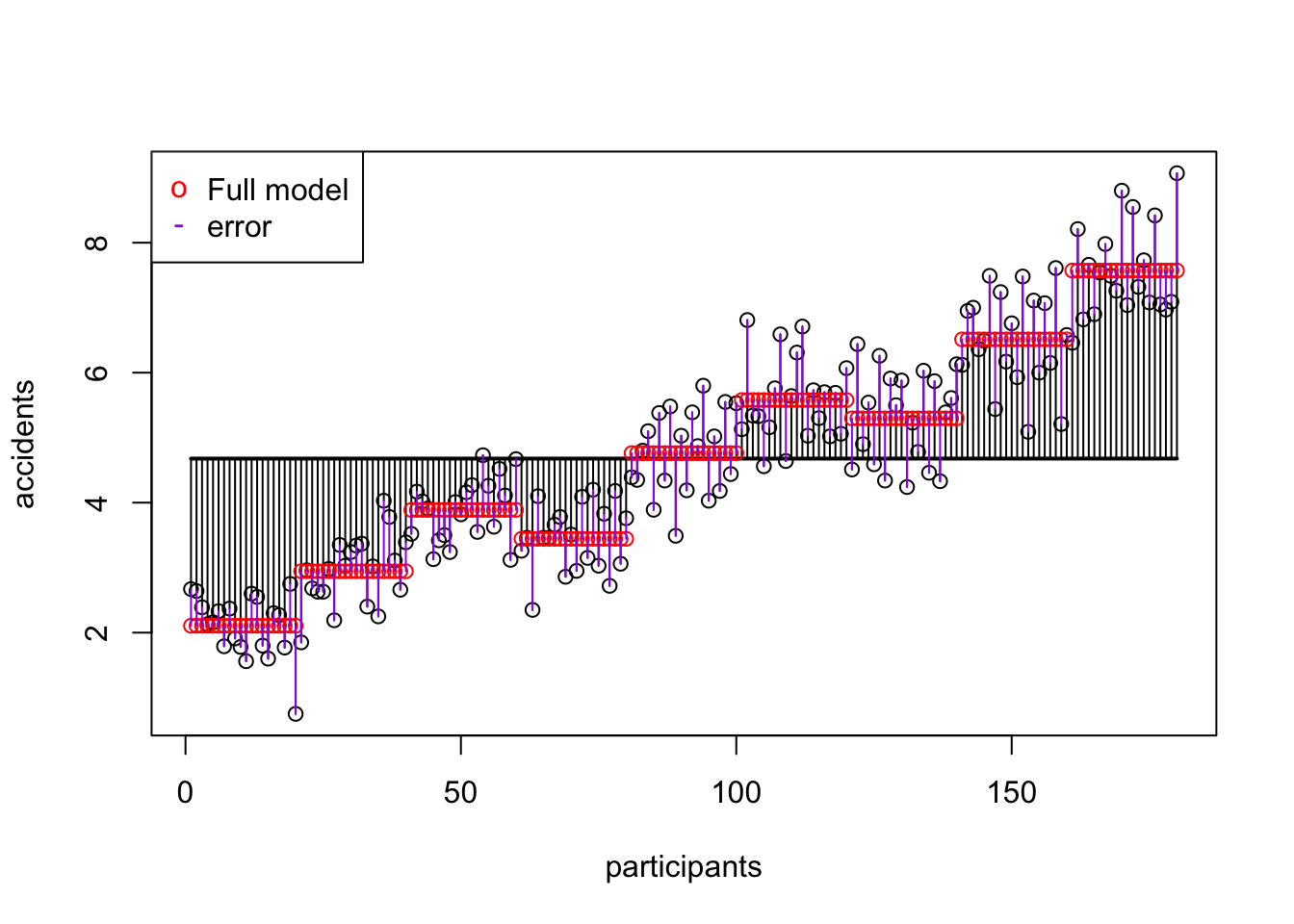
SS error

\(\text{SS}_\text{error} = 66.34642\)

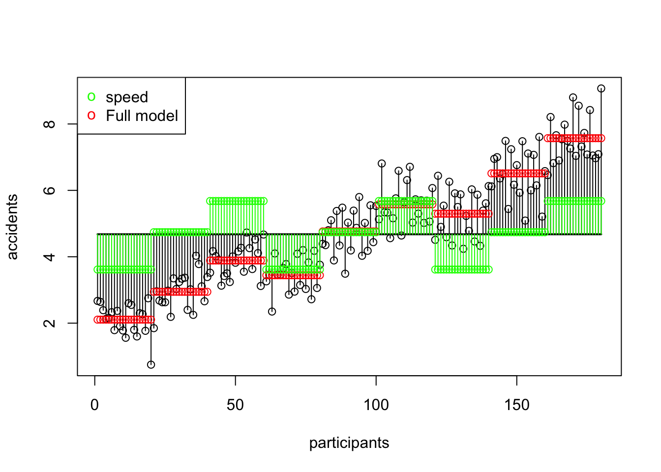
SS A Speed

\(\text{SS}_\text{speed} = 128.1639233\)

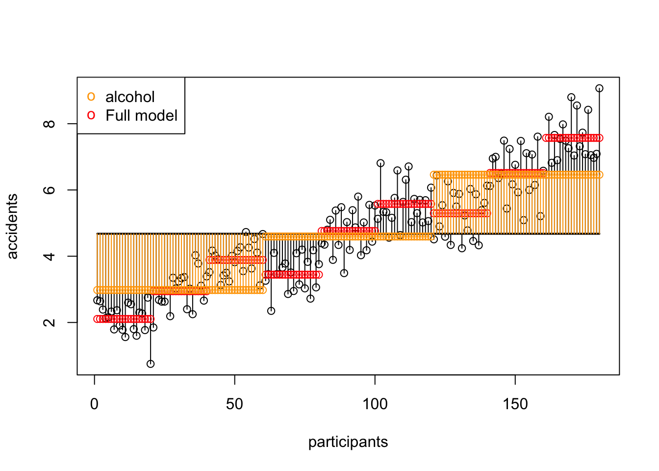
SS B Alcohol

\(\text{SS}_\text{alcohol} = 364.14583\)

SS AB Alcohol x Speed

Variance	Sum of squares	df	Mean squares	F-ratio
\(\hspace{2ex}AB\)	\(\text{SS}_{A \times B} = \text{SS}_{\text{model}} - \text{SS}_{\text{A}} - \text{SS}_{\text{B}}\)	\(df_A \times df_B\)	\(\frac{\text{SS}_{\text{AB}}}{\text{df}_{\text{AB}}}\)	\(\frac{\text{MS}_{\text{AB}}}{\text{MS}_{\text{error}}}\)

\[\text{SS}_{\text{speed} \times \text{alcohol}} = 1.9107267\]

Mean Squares

Mean squares for:

Speed
Alcohol
Speed \(\times\) Alcohol

\[\begin{aligned} F_{Speed} &= \frac{{MS}_{Speed}}{{MS}_{error}} \\ F_{Alcohol} &= \frac{{MS}_{Alcohol}}{{MS}_{error}} \\ F_{Alcohol \times Speed} &= \frac{{MS}_{Alcohol \times Speed}}{{MS}_{error}} \\ \end{aligned}\]

Interaction

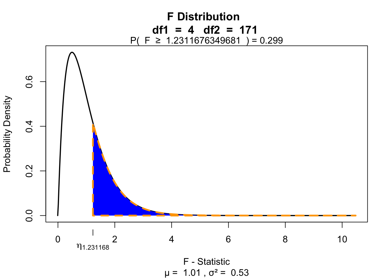
\[F_{Alcohol \times Speed} = \frac{{MS}_{Alcohol \times Speed}}{{MS}_{error}} = \frac{0.48}{0.39} = 1.23\]

\(P\)-value

Post-Hoc

Unplanned comparisons

Exploring all possible differences
Adjust T value for inflated type 1 error

Effect size

General effect size measures

Amount of explained variance \(R^2\) also called eta squared \(\eta^2\).

Effect sizes of post-hoc comparisons

Cohen’s \(r\) gives the effect size for a specific comparison
- \(r_{Contrast} = \sqrt{\frac{t^2}{t^2+{df}}}\)

ANOVA as regression

Linear line equation

\(Y = aX + b\)

Regression equation

\[\text{outcome} = \text{model} + \text{error}\]

\[\text{model} = b_0 + b_1 \times \text{predictor}\]

Data

Aalcohol + Weight

\[\text{outcome} = \text{model} + \text{error}\]

\[\text{model}\]

\[b_0 + b_1 \times \text{alcohol} + b_2 \times \text{weight}\]

Dummies

Categorical variable need to be recoded into \([0, 1]\) (on / off) dummy variables. Number of categories - 1 dummies.

alcohol [none, some, much]
- none \([0,1]\)
- some \([0,1]\)

\(b_0 + b_1 \times \text{none alcohol} + b_2 \times \text{some alcohol} + b_3 \times \text{weight}\)

Aalcohol x Weight

\[ \begin{aligned} b_0 & + b_1 \times \text{none alcohol} \\ & + b_2 \times \text{some alcohol} \\ & + b_3 \times \text{weight} \\ & + b_4 \times \text{none alcohol} \times \text{weight} \\ & + b_5 \times \text{some alcohol} \times \text{weight} \\ \end{aligned} \]

Regression model

\[ \begin{aligned} 21.325 & + -17.831 \times \text{none}_{01} \\ & + -0.512 \times \text{some}_{01} \\ & + -0.216 \times \text{weight} \\ & + 0.208 \times \text{none}_{01} \times \text{weight} \\ & + 0.004 \times \text{some}_{01} \times \text{weight} \\ \end{aligned} \]

Data with dummies

\(\tiny 21.325 + -17.831 \times \text{none}_{01} + -0.512 \times \text{some}_{01} + -0.216 \times \text{weight} + 0.208 \times \text{none}_{01} \times \text{weight} + 0.004 \times \text{some}_{01} \times \text{weight}\)

How good is the model

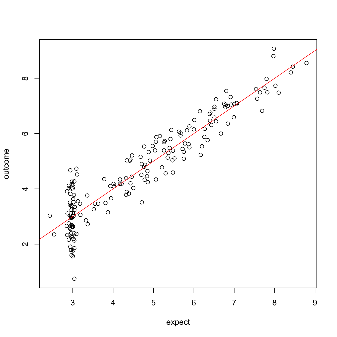
\[\LARGE \eta^2\]

Squared correlation between model expectation and actual outcome: 0.873

Proportion of:

explained / total variance
model / total variance
between group variance / total variance.

\(\frac{489.613}{560.567} = 0.873\)

End

Contact