Multiple regression
Klinkenberg
16 sep 2020
Inhoud
### Outline
- 0:00 Test analysis
- 0:40 Regression
- 1:00 Example in SPSS (enter method with 2 blocks)
- 1:20 Regression slides (regression plane)
T-distribution
Gosset

In probability and statistics, Student’s t-distribution (or simply the t-distribution) is any member of a family of continuous probability distributions that arises when estimating the mean of a normally distributed population in situations where the sample size is small and population standard deviation is unknown.
In the English-language literature it takes its name from William Sealy Gosset’s 1908 paper in Biometrika under the pseudonym “Student”. Gosset worked at the Guinness Brewery in Dublin, Ireland, and was interested in the problems of small samples, for example the chemical properties of barley where sample sizes might be as low as 3.
Source: Wikipedia

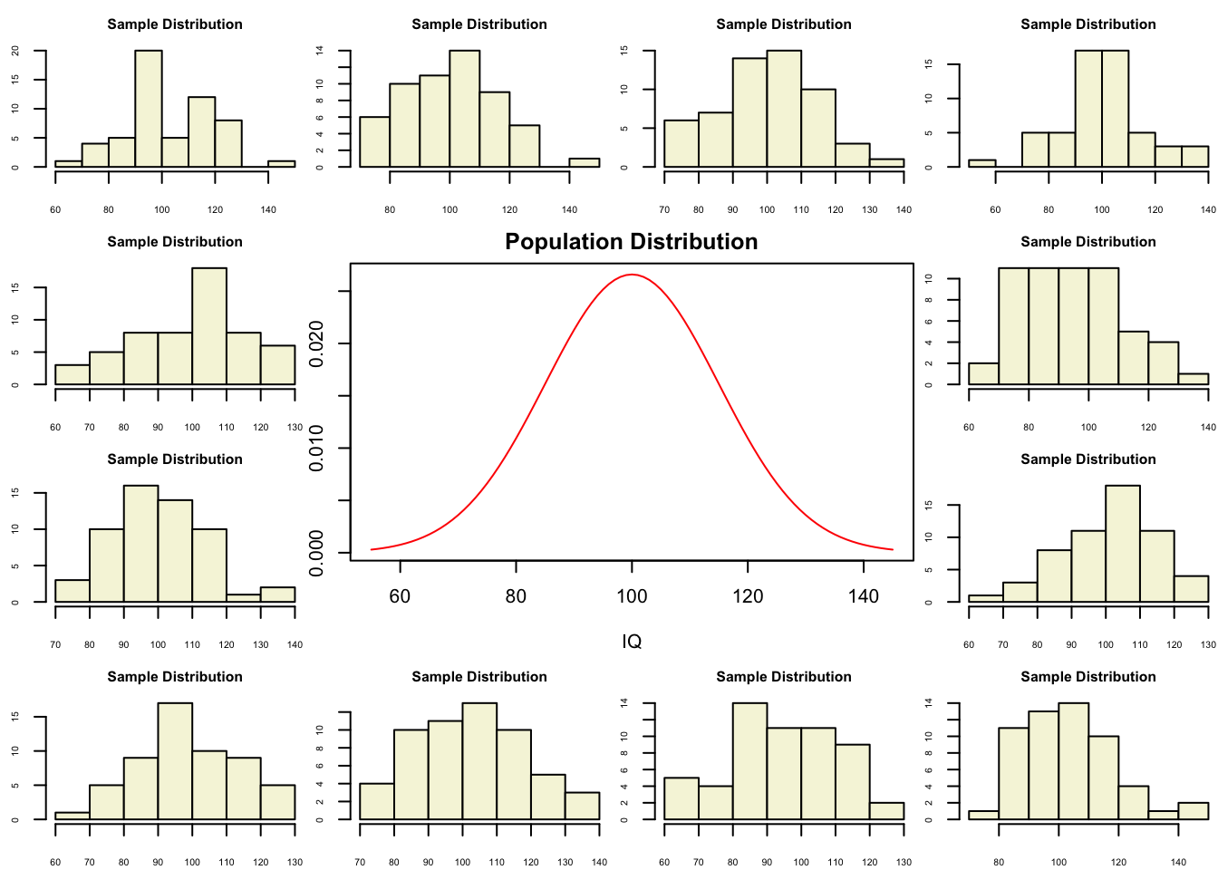
Population distribution
layout(matrix(c(2:6,1,1,7:8,1,1,9:13), 4, 4))

n  = 56    # Sample size
df = n - 1 # Degrees of freedom

mu    = 100
sigma = 15

IQ = seq(mu-45, mu+45, 1)

par(mar=c(4,2,2,0))
plot(IQ, dnorm(IQ, mean = mu, sd = sigma), type='l', col="red", main = "Population Distribution")

n.samples = 12

for(i in 1:n.samples) {

  par(mar=c(2,2,2,0))
  hist(rnorm(n, mu, sigma), main="Sample Distribution", cex.axis=.5, col="beige", cex.main = .75)

}
T-statistic
\[T_{n-1} = \frac{\bar{x}-\mu}{SE_x} = \frac{\bar{x}-\mu}{s_x / \sqrt{n}}\]
So the t-statistic represents the deviation of the sample mean \(\bar{x}\) from the population mean \(\mu\), considering the sample size, expressed as the degrees of freedom \(df = n - 1\)
A sample
Let’s take one sample from our normal populatiion and calculate the t-value.
x = rnorm(n, mu, sigma); x## [1] 103.80813 102.74285 78.67846 99.91030 98.55335 99.90442 127.60760 82.51476
## [9] 99.51833 96.63494 136.51783 118.40084 88.60622 90.04249 108.53620 103.96831
## [17] 108.51006 98.94223 81.88491 119.60836 111.44797 86.63278 93.41979 114.93519
## [25] 116.70249 111.32529 117.15964 108.71884 120.28769 80.96595 103.14218 111.74893
## [33] 109.89408 99.91094 119.82214 83.77042 117.10553 114.83815 90.81676 97.86342
## [41] 71.38087 95.17512 123.86021 109.56622 100.25551 103.64829 125.70421 97.79102
## [49] 86.04313 110.08855 88.55775 120.19644 125.30307 73.43386 103.75659 104.11733hist(x, main = "Sample distribution", col = "beige")
text(80, 10, round(mean(x),2))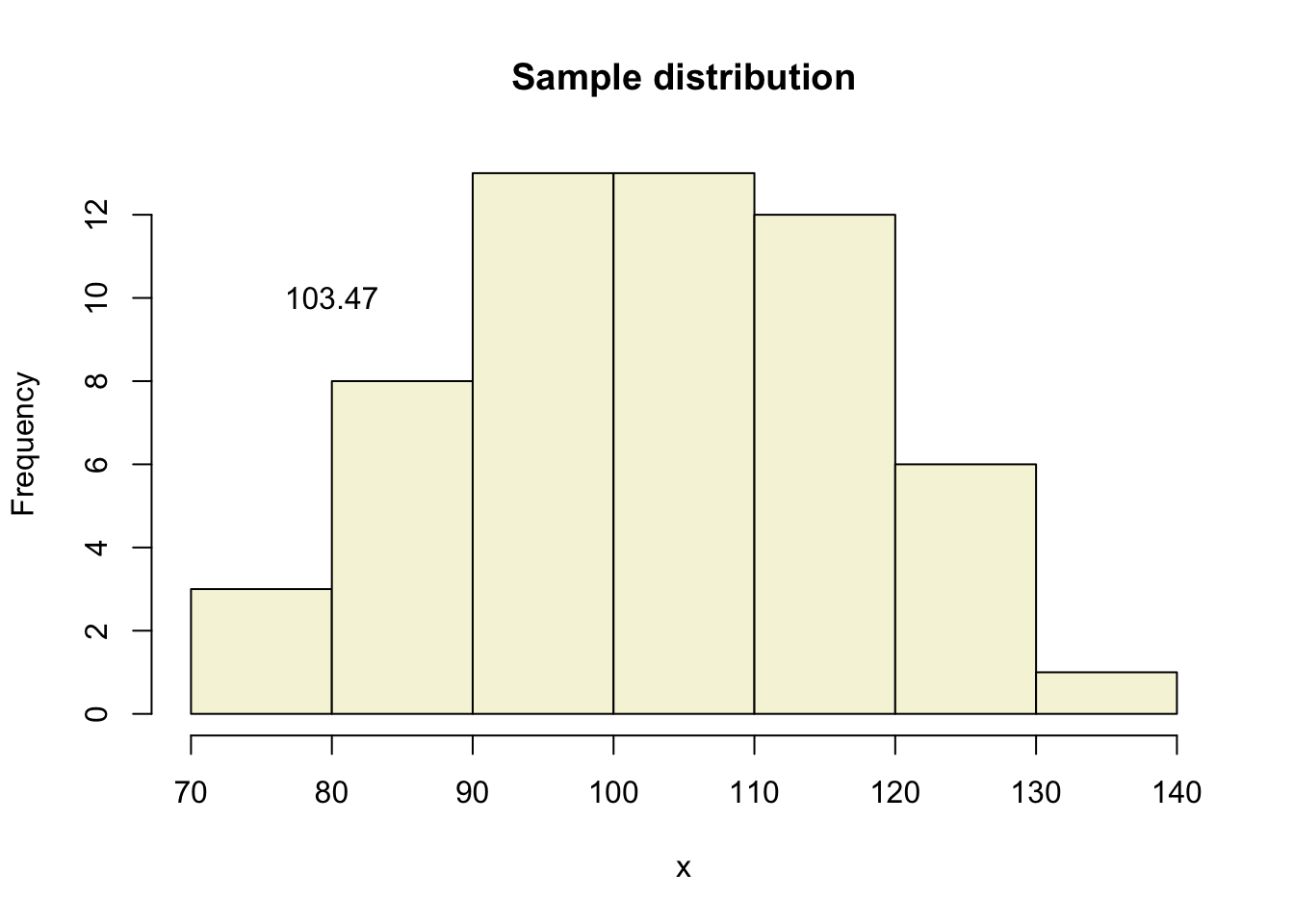
t-value
\[T_{n-1} = \frac{\bar{x}-\mu}{SE_x} = \frac{\bar{x}-\mu}{s_x / \sqrt{n}}\]
t = (mean(x) - mu) / (sd(x) / sqrt(n))
t
## [1] 1.781033More samples
let’s take more samples.
n.samples     = 1000
mean.x.values = vector()
se.x.values   = vector()

for(i in 1:n.samples) {
  x = rnorm(n, mu, sigma)
  mean.x.values[i] = mean(x)
  se.x.values[i]   = (sd(x) / sqrt(n))
}
Mean and SE for all samples
head(cbind(mean.x.values, se.x.values))## mean.x.values se.x.values
## [1,] 100.94192 2.197250
## [2,] 99.16970 1.818559
## [3,] 99.96827 1.893275
## [4,] 100.17359 2.241665
## [5,] 99.27712 1.988195
## [6,] 100.08231 2.072537Sampling distribution
hist(mean.x.values,
     col  = "beige",
     main = "Sampling distribution",
     xlab = "all sample means")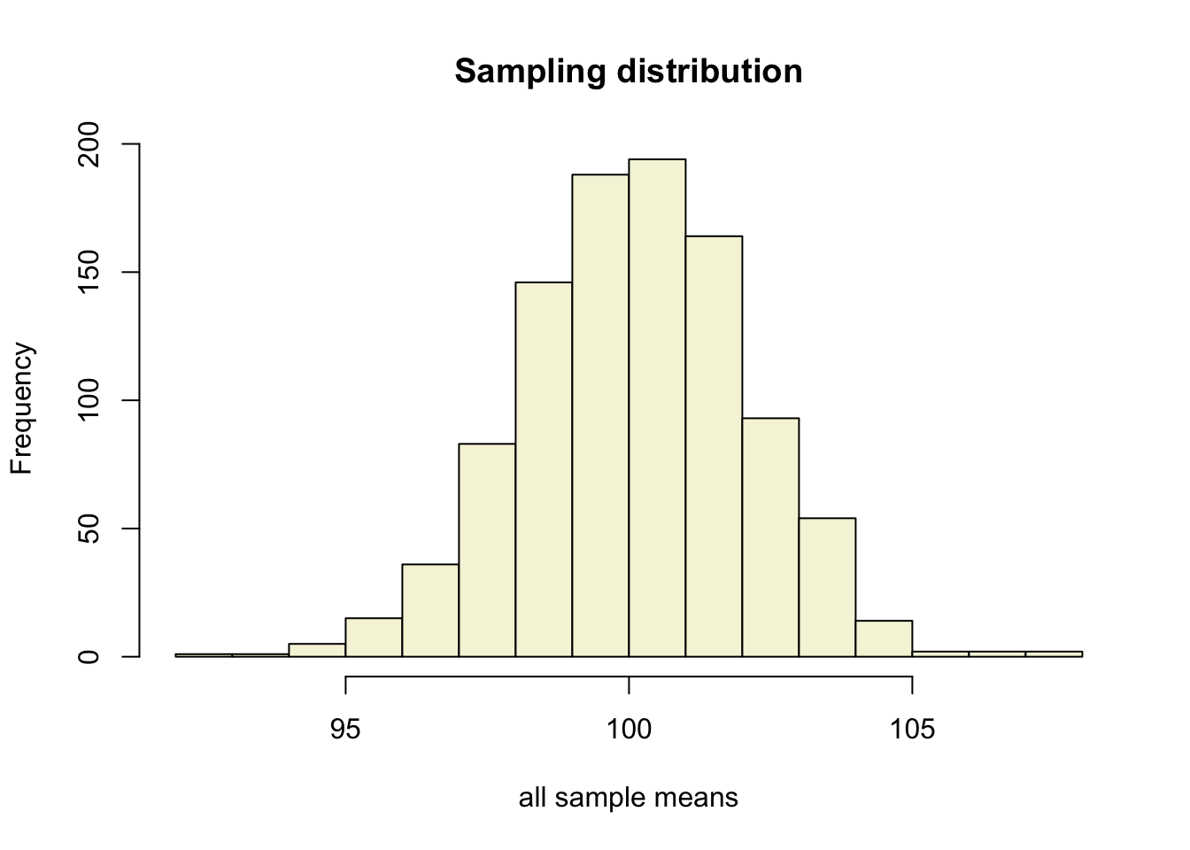
Calculate t-values
\[T_{n-1} = \frac{\bar{x}-\mu}{SE_x} = \frac{\bar{x}-\mu}{s_x / \sqrt{n}}\]
t.values = (mean.x.values - mu) / se.x.values

tail(cbind(mean.x.values, mu, se.x.values, t.values))
## mean.x.values mu se.x.values t.values
## [995,] 96.63986 100 1.965583 -1.7094880
## [996,] 101.30901 100 2.331382 0.5614726
## [997,] 100.28059 100 1.645908 0.1704749
## [998,] 98.72011 100 1.872404 -0.6835541
## [999,] 99.56572 100 1.814711 -0.2393136
## [1000,] 99.11019 100 1.724447 -0.5159949Sampled t-values
What is the distribution of all these t-values?
hist(t.values,
     freq = F,
     main = "Sampled T-values",
     xlab = "T-values",
     col  = "beige",
     ylim = c(0, .4))
T = seq(-4, 4, .01)
lines(T, dt(T,df), col = "red")
legend("topright", lty = 1, col="red", legend = "T-distribution")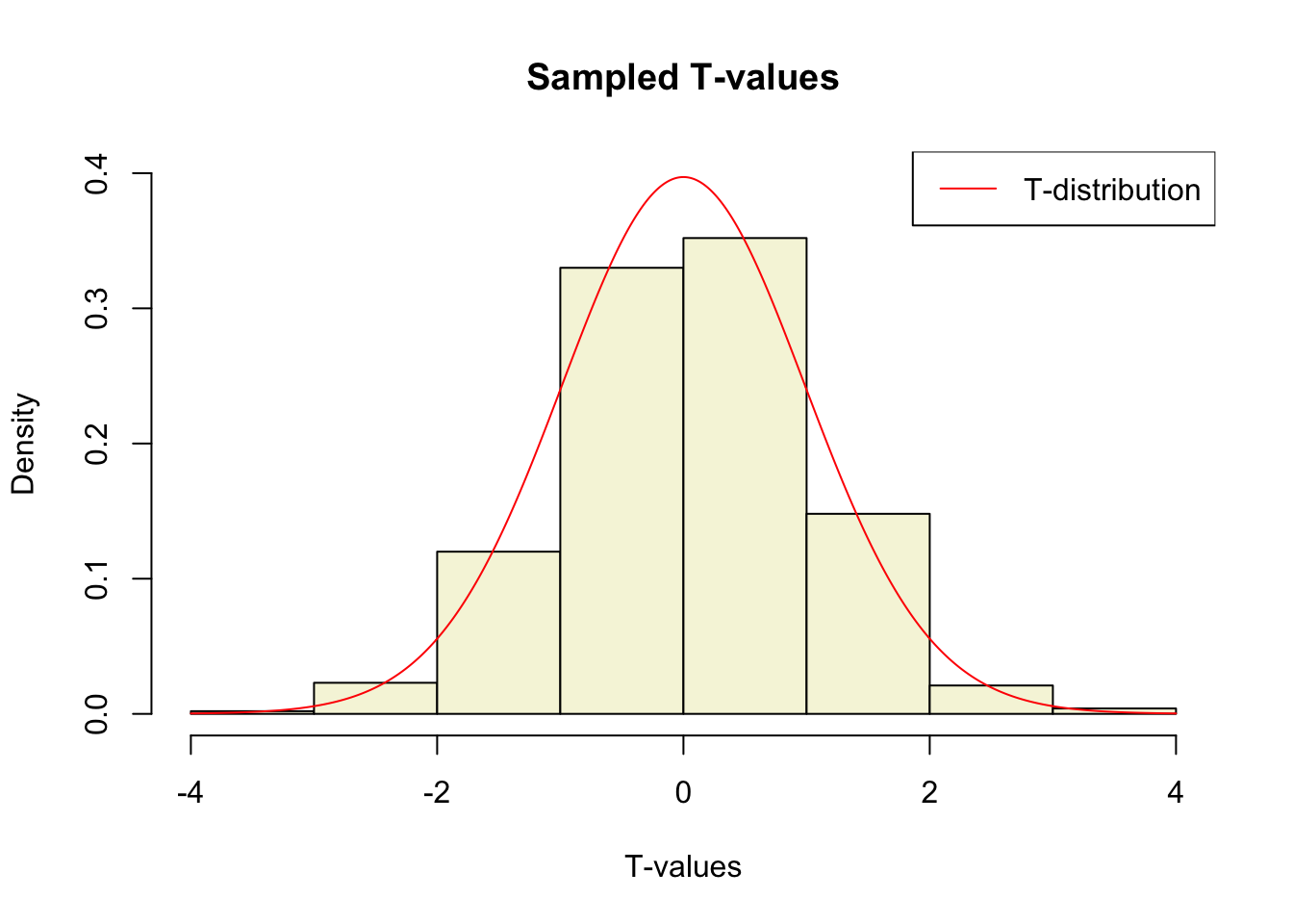
T-distribution
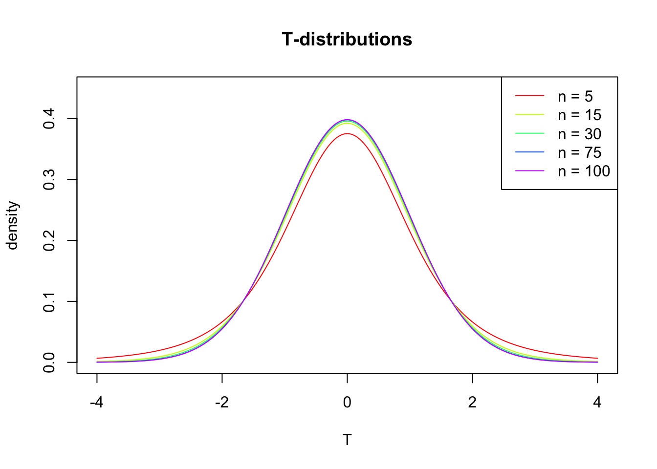
So if the population is normaly distributed (assumption of normality) the t-distribution represents the deviation of sample means from the population mean (\(\mu\)), given a certain sample size (\(df = n - 1\)).
The t-distibution therefore is different for different sample sizes and converges to a standard normal distribution if sample size is large enough.
The t-distribution is defined by:
\[\textstyle\frac{\Gamma \left(\frac{\nu+1}{2} \right)} {\sqrt{\nu\pi}\,\Gamma \left(\frac{\nu}{2} \right)} \left(1+\frac{x^2}{\nu} \right)^{-\frac{\nu+1}{2}}\!\]
where \(\nu\) is the number of degrees of freedom and \(\Gamma\) is the gamma function.
Source: wikipedia
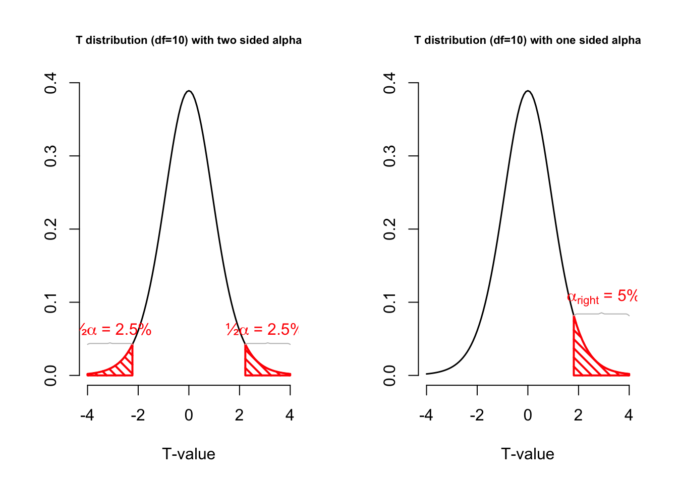
One or two sided
Two sided
- \(H_A: \bar{x} \neq \mu\)
One sided
- \(H_A: \bar{x} > \mu\)
- \(H_A: \bar{x} < \mu\)
Effect-size
The effect-size is the standardised difference between the mean and the expected \(\mu\). In the t-test effect-size is expressed as \(r\).
\[r = \sqrt{\frac{t^2}{t^2 + \text{df}}}\]
r = sqrt(t^2/(t^2 + df))

r
## [1] 0.2603778Effect-size distribution
We can also calculate effect-sizes for all our calculated t-values. Under the assumption of \(H_0\) the effect-size distribution looks like this.
r = sqrt(t.values^2/(t.values^2 + df))

tail(cbind(mean.x.values, mu, se.x.values, t.values, r))
## mean.x.values mu se.x.values t.values r
## [995,] 96.63986 100 1.965583 -1.7094880 0.22461718
## [996,] 101.30901 100 2.331382 0.5614726 0.07549290
## [997,] 100.28059 100 1.645908 0.1704749 0.02298076
## [998,] 98.72011 100 1.872404 -0.6835541 0.09178138
## [999,] 99.56572 100 1.814711 -0.2393136 0.03225225
## [1000,] 99.11019 100 1.724447 -0.5159949 0.06940894hist(r, main = "effect-size distribution", col = "beige")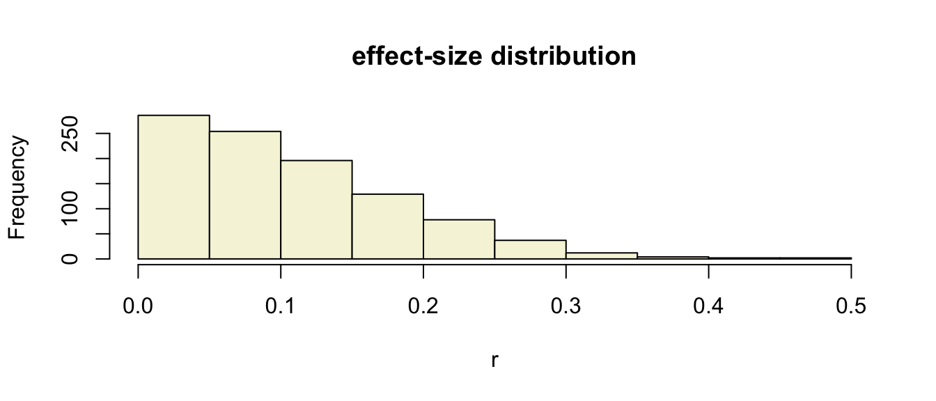
Cohen (1988)
- Small: 0 <= .1
- Medium: .1 <= .3
- Large: .3 <= .5
Power
- Strive for 80%
- Based on know effect size
- Calculate number of subjects needed
- Use G*Power to calculate

Alpha Power
T = seq(-3,6,.01)
N = 45
E = 2

# Set plot
plot(0,0,
     type = "n",
     ylab = "Density",
     xlab = "T",
     ylim = c(0,.5),
     xlim = c(-3,6),
     main = "T-Distributions under H0 and HA")

critical_t = qt(.05,N-1,lower.tail=FALSE)

# Alpha
range_x = seq(critical_t,6,.01)
polygon(c(range_x,rev(range_x)),
        c(range_x*0,rev(dt(range_x,N-1,ncp=0))),
        col     = "grey",
        density = 10,
        angle   = 90,
        lwd     = 2)

# Power
range_x = seq(critical_t,6,.01)
polygon(c(range_x,rev(range_x)),
        c(range_x*0,rev(dt(range_x,N-1,ncp=E))),
        col     = "grey",
        density = 10,
        angle   = 45,
        lwd     = 2)

lines(T,dt(T,N-1,ncp=0),col="red", lwd=2) # H0 line
lines(T,dt(T,N-1,ncp=E),col="blue",lwd=2) # HA line

# Critical value
lines(rep(critical_t,2),c(0,dt(critical_t,N-1,ncp=E)),lwd=2,col="black")
text(critical_t,dt(critical_t,N-1,ncp=E),"critical T-value",pos=2, srt = 90)

# H0 and HA
text(0,dt(0,N-1,ncp=0),expression(H[0]),pos=3,col="red", cex=2)
text(E,dt(E,N-1,ncp=E),expression(H[A]),pos=3,col="blue",cex=2)

# Mu H0 line
lines(c(0,0),c(0,dt(0,N-1)), col="red",  lwd=2,lty=2)
text(0,dt(0,N-1,ncp=0)/2,expression(mu),pos=4,cex=1.2)
# Mu HA line
lines(c(E,E),c(0,dt(E,N-1,ncp=E)),col="blue",lwd=2,lty=2)
text(E,dt(0,N-1,ncp=0)/2,expression(paste(mu)),pos=4,cex=1.2)

# t-value
lines( c(critical_t+.01,6),c(0,0),col="green",lwd=4)

# Legend
legend("topright", c(expression(alpha),'POWER'),density=c(10,10),angle=c(90,45))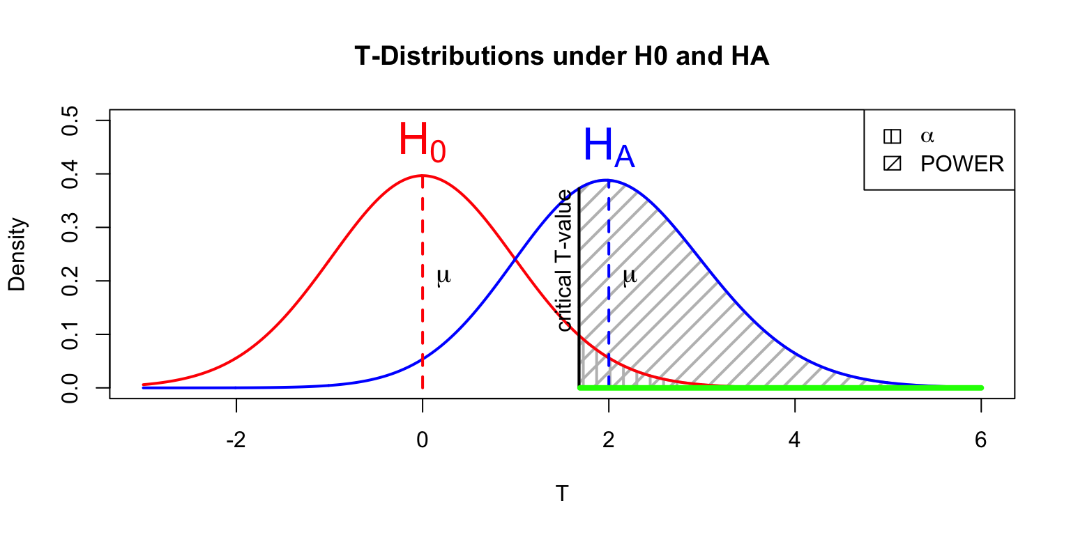
Multiple regression
Multiple regression
\[\LARGE{\text{outcome} = \text{model} + \text{error}}\]
In statistics, linear regression is a linear approach for modeling the relationship between a scalar dependent variable y and one or more explanatory variables denoted X.
\[\LARGE{Y_i = \beta_0 + \beta_1 X_{1i} + \beta_2 X_{2i} + \dotso + \beta_n X_{ni} + \epsilon_i}\]
In linear regression, the relationships are modeled using linear predictor functions whose unknown model parameters \(\beta\)’s are estimated from the data.
Source: wikipedia
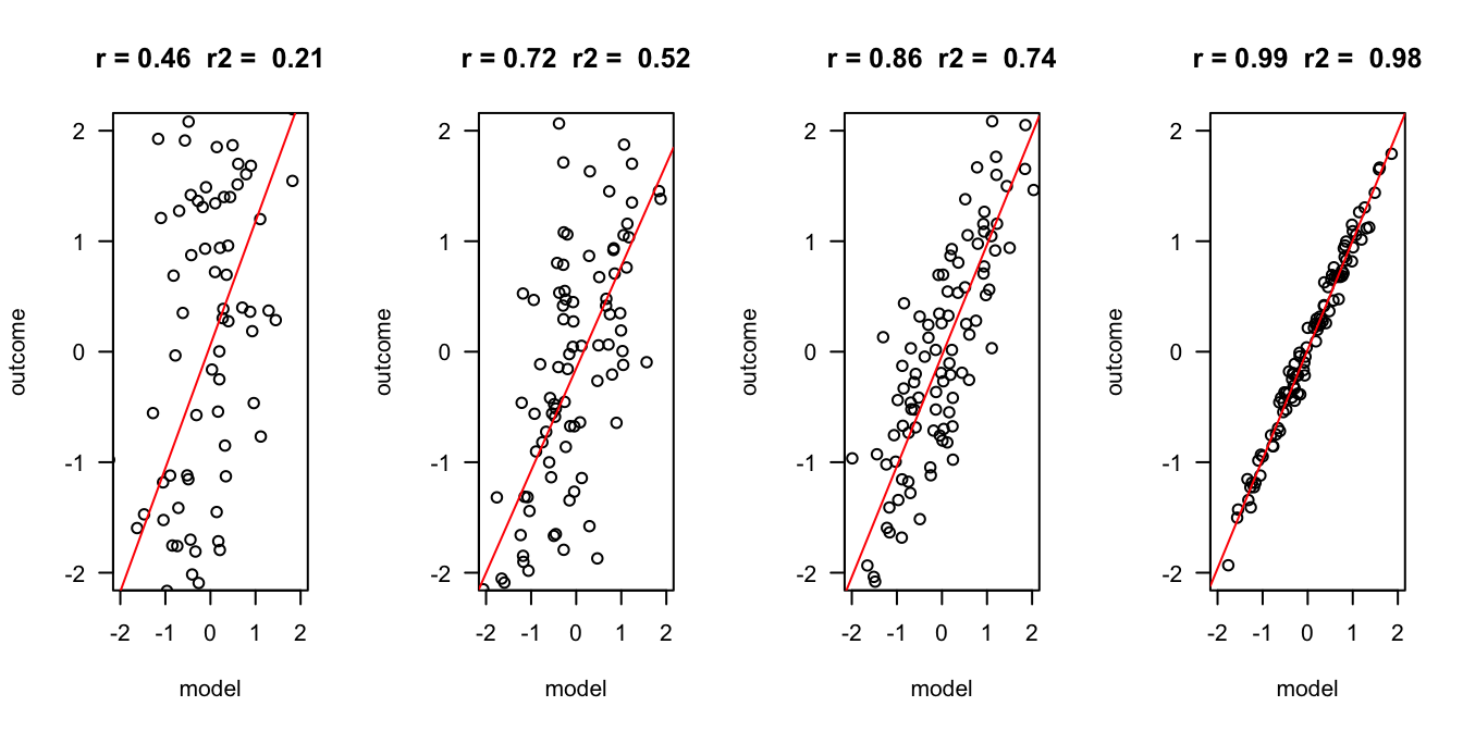
Outcome vs Model
error = c(2, 1, .5, .1)
n = 100

layout(matrix(1:4,1,4))
for(e in error) {

  x = rnorm(n)
  y = x + rnorm(n, 0 , e)

  r   = round(cor(x,y), 2)
  r.2 = round(r^2, 2)

  plot(x,y, las = 1, ylab = "outcome", xlab = "model", main = paste("r =", r," r2 = ", r.2), ylim=c(-2,2), xlim=c(-2,2))
  fit <- lm(y ~ x)
  abline(fit, col = "red")

}
Assumptions
A selection from Field (8.3.2.1. Assumptions of the linear model):
For simple regression
- Sensitivity
- Homoscedasticity
For multiple regressin
- Multicollinearity
- Linearity
Sensitivity
Outliers
- Extreme residuals
- Cook’s distance (< 1)
- Mahalonobis (< 11 at N = 30)
- Laverage (The average leverage value is defined as (k + 1)/n)
Homoscedasticity
- Variance of residual should be equal across all expected values
- Look at scatterplot of standardized: expected values \(\times\) residuals. Roughly round shape is needed.
fit <- lm(x[2:n] ~ y[2:n])

ZPRED  = scale(fit$fitted.values)
ZREDID = scale(fit$residuals)

plot(ZPRED, ZREDID)
abline(h = 0, v = 0, lwd=2)

#install.packages("plotrix")
if(!"plotrix" %in% installed.packages()) { install.packages("plotrix") };
library("plotrix")
draw.circle(0,0,1.7,col=rgb(1,0,0,.5))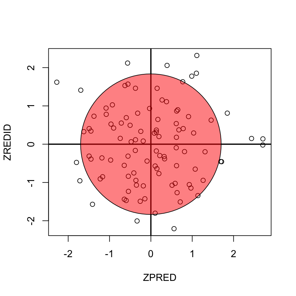
Multicollinearity

To adhere to the multicollinearity assumptien, there must not be a too high linear relation between the predictor variables.
This can be assessed through:
- Correlations
- Matrix scatterplot
- Tolerance > 0.2
Linearity
For the linearity assumption to hold, the predictors must have a linear relation to the outcome variable.
This can be checked through:
- Correlations
- Matrix scatterplot with predictors and outcome variable
Example
Perdict study outcome based on IQ and motivation.
Read data
# data <- read.csv('IQ.csv', header=T)
data <- read.csv('http://shklinkenberg.github.io/statistics-lectures/topics/regression_multiple_predictors/IQ.csv', header=T)
head(data)
## Studieprestatie Motivatie IQ
## 1 2.710330 3.276778 129.9922
## 2 2.922617 2.598901 128.4936
## 3 1.997056 3.207279 130.2709
## 4 2.322539 2.104968 125.7457
## 5 2.162133 3.264948 128.6770
## 6 2.278899 2.217771 127.5349IQ = data$IQ
study.outcome = data$Studieprestatie
motivation = data$MotivatieRegression model in R
Perdict study outcome based on IQ and motivation.
fit <- lm(study.outcome ~ IQ + motivation)What is the model
fit$coefficients## (Intercept) IQ motivation
## -30.2822189 0.2690984 -0.6314253b.0 = round(fit$coefficients[1], 2) ## Intercept
b.1 = round(fit$coefficients[2], 2) ## Beta coefficient for IQ
b.2 = round(fit$coefficients[3], 2) ## Beta coefficient for motivationDe beta coëfficients are:
- \(b_0\) (intercept) = -30.28
- \(b_1\) = 0.27
- \(b_2\) = -0.63.
Model summaries
summary(fit)##
## Call:
## lm(formula = study.outcome ~ IQ + motivation)
##
## Residuals:
## Min 1Q Median 3Q Max
## -0.75127 -0.17437 0.00805 0.17230 0.44435
##
## Coefficients:
## Estimate Std. Error t value Pr(>|t|)
## (Intercept) -30.28222 6.64432 -4.558 5.76e-05 ***
## IQ 0.26910 0.05656 4.758 3.14e-05 ***
## motivation -0.63143 0.23143 -2.728 0.00978 **
## ---
## Signif. codes: 0 '***' 0.001 '**' 0.01 '*' 0.05 '.' 0.1 ' ' 1
##
## Residual standard error: 0.2714 on 36 degrees of freedom
## Multiple R-squared: 0.7528, Adjusted R-squared: 0.739
## F-statistic: 54.8 on 2 and 36 DF, p-value: 1.192e-11Visual
What are the expected values based on this model
\[\widehat{\text{studie prestatie}} = b_0 + b_1 \text{IQ} + b_2 \text{motivation}\]
exp.stu.prest = b.0 + b.1 * IQ + b.2 * motivation

model = exp.stu.prest
\[\text{model} = \widehat{\text{studie prestatie}}\]
Apply regression model
\[\widehat{\text{studie prestatie}} = b_0 + b_1 \text{IQ} + b_2 \text{motivation}\] \[\widehat{\text{model}} = b_0 + b_1 \text{IQ} + b_2 \text{motivation}\]
cbind(model, b.0, b.1, IQ, b.2, motivation)[1:5,]## model b.0 b.1 IQ b.2 motivation
## [1,] 2.753512 -30.28 0.27 129.9922 -0.63 3.276778
## [2,] 2.775969 -30.28 0.27 128.4936 -0.63 2.598901
## [3,] 2.872561 -30.28 0.27 130.2709 -0.63 3.207279
## [4,] 2.345205 -30.28 0.27 125.7457 -0.63 2.104968
## [5,] 2.405860 -30.28 0.27 128.6770 -0.63 3.264948\[\widehat{\text{model}} = -30.28 + 0.27 \times \text{IQ} + -0.63 \times \text{motivation}\]
How far are we off?
error = study.outcome - model

cbind(model, study.outcome, error)[1:5,]
## model study.outcome error
## [1,] 2.753512 2.710330 -0.04318159
## [2,] 2.775969 2.922617 0.14664823
## [3,] 2.872561 1.997056 -0.87550534
## [4,] 2.345205 2.322539 -0.02266610
## [5,] 2.405860 2.162133 -0.24372667Outcome = Model + Error
Is that true?
study.outcome == model + error## [1] TRUE TRUE TRUE TRUE TRUE TRUE TRUE TRUE TRUE TRUE TRUE TRUE TRUE TRUE TRUE TRUE
## [17] TRUE TRUE TRUE TRUE TRUE TRUE TRUE TRUE TRUE TRUE TRUE TRUE TRUE TRUE TRUE TRUE
## [33] TRUE TRUE TRUE TRUE TRUE TRUE TRUE
- Yes!
Visual
plot(study.outcome, xlab='personen', ylab='study.outcome')

n = length(study.outcome)
gemiddelde.study.outcome = mean(study.outcome)

## Voeg het gemiddelde toe
lines(c(1, n), rep(gemiddelde.study.outcome, 2))

## Wat is de totale variantie?
segments(1:n, study.outcome, 1:n, gemiddelde.study.outcome, col='blue')

## Wat zijn onze verwachte scores op basis van dit regressie model?
points(model, col='orange')

## Hoever zitten we ernaast, wat is de error?
segments(1:n, study.outcome, 1:n, model, col='purple', lwd=3)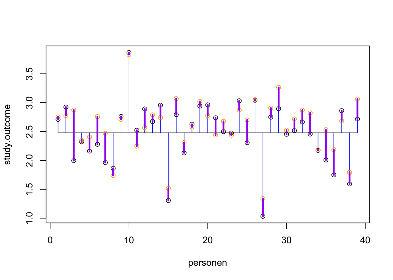
Explained variance
The explained variance is the deviation of the estimated model outcome compared to the total mean.
To get a percentage of explained variance, it must be compared to the total variance. In terms of squares:
\[\frac{{SS}_{model}}{{SS}_{total}}\]
We also call this: \(r^2\) of \(R^2\).
r = cor(study.outcome, model)
r^2
## [1] 0.7527463Compare models
fit1 <- lm(study.outcome ~ motivation, data)
fit2 <- lm(study.outcome ~ motivation + IQ, data)

# summary(fit1)
# summary(fit2)

anova(fit1, fit2)
## Analysis of Variance Table
##
## Model 1: study.outcome ~ motivation
## Model 2: study.outcome ~ motivation + IQ
## Res.Df RSS Df Sum of Sq F Pr(>F)
## 1 37 4.3191
## 2 36 2.6518 1 1.6673 22.635 3.144e-05 ***
## ---
## Signif. codes: 0 '***' 0.001 '**' 0.01 '*' 0.05 '.' 0.1 ' ' 1